data("penguins", package = "palmerpenguins")
pg <- penguins |>
  filter(species %in% c("Adelie", "Gentoo")) |>
  mutate(species = droplevels(species)) |>
  tidyr::drop_na()
table(pg$species)
Adelie Gentoo
146 119 This notebook uses Palmer Penguins for classification. We use a binary task — Adelie vs Gentoo — after dropping Chinstrap (cleaner boundaries in 2D plots; for three species see penguins-species-multiclass.Rmd).
Models: glm logistic regression and an rpart tree. Splits and metrics: tidymodels / yardstick (conf_mat).
Same scientific task with tidymodels: preprocessing + workflow + resampling live on the website in Module 04 (starts with train/test + glm, then the Tuesday tuned-tree pipeline), with follow-ups Module 07 (pick a metric) and Module 08 (compare RF / XGBoost / MLP).
The synthetic gene / disease notebook (logistic-regression-gene-disease.Rmd) stays the place for known-truth logistic stories.
data("penguins", package = "palmerpenguins")
pg <- penguins |>
filter(species %in% c("Adelie", "Gentoo")) |>
mutate(species = droplevels(species)) |>
tidyr::drop_na()
table(pg$species)
Adelie Gentoo
146 119 GGally::ggpairs(
pg,
columns = c("bill_length_mm", "bill_depth_mm", "flipper_length_mm", "body_mass_g", "sex"),
aes(color = species)
) +
theme_minimal()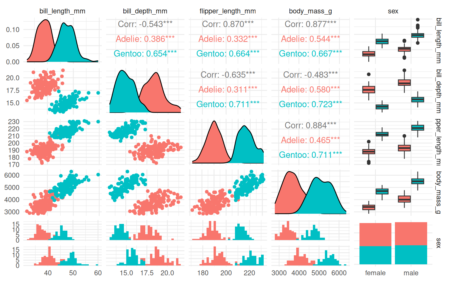
log_fit <- glm(
  species ~ bill_length_mm + bill_depth_mm + flipper_length_mm + body_mass_g + island + sex,
  data = pg,
  family = binomial()
)
summary(log_fit)
Call:
glm(formula = species ~ bill_length_mm + bill_depth_mm + flipper_length_mm +
    body_mass_g + island + sex, family = binomial(), data = pg)

Coefficients:
                    Estimate Std. Error z value Pr(>|z|)
(Intercept)       -1.448e+02  1.068e+06       0        1
bill_length_mm     1.239e+00  1.141e+04       0        1
bill_depth_mm     -9.516e+00  2.768e+04       0        1
flipper_length_mm  9.082e-01  3.216e+03       0        1
body_mass_g        1.410e-02  6.212e+01       0        1
islandDream       -5.630e+00  6.667e+04       0        1
islandTorgersen   -1.118e+01  7.399e+04       0        1
sexmale            2.906e+00  1.221e+05       0        1

(Dispersion parameter for binomial family taken to be 1)

    Null deviance: 3.6461e+02  on 264  degrees of freedom
Residual deviance: 5.1900e-09  on 257  degrees of freedom
AIC: 16

Number of Fisher Scoring iterations: 25tree_fit <- rpart(
species ~ bill_length_mm + bill_depth_mm + flipper_length_mm + body_mass_g + island + sex,
data = pg,
method = "class"
)
rpart.plot(tree_fit, type = 4, extra = 104, main = "Adelie vs Gentoo (rpart)")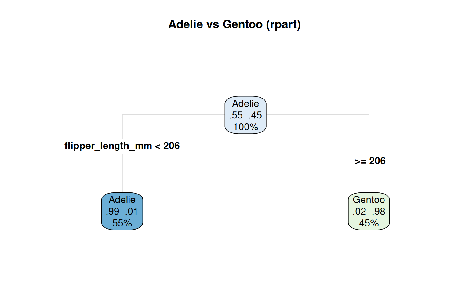
pred_class <- predict(tree_fit, type = "class")
tibble(truth = pg$species, .pred_class = pred_class) |>
  conf_mat(truth = truth, estimate = .pred_class)
Truth
Prediction Adelie Gentoo
Adelie 144 1
Gentoo 2 118Other predictors held at their training means / modes.
plot_boundary <- function(model, data, f1, f2) {
  r1 <- range(data[[f1]])
  r2 <- range(data[[f2]])
  grid <- expand.grid(
    seq(r1[1], r1[2], length.out = 120),
    seq(r2[1], r2[2], length.out = 120)
  )
  names(grid) <- c(f1, f2)
  for (nm in setdiff(names(data), c(f1, f2, "species"))) {
    v <- data[[nm]]
    grid[[nm]] <- if (is.numeric(v)) {
      mean(v, na.rm = TRUE)
    } else {
      tab <- table(v)
      grid[[nm]] <- names(tab)[which.max(tab)]
    }
  }
  grid$p_Gentoo <- predict(model, newdata = grid, type = "response")
  grid$cls <- factor(ifelse(grid$p_Gentoo > 0.5, "Gentoo", "Adelie"), levels = c("Adelie", "Gentoo"))
  ggplot(data, aes(!!sym(f1), !!sym(f2))) +
    geom_raster(data = grid, aes(!!sym(f1), !!sym(f2), fill = cls), alpha = 0.25, inherit.aes = FALSE) +
    geom_point(aes(shape = species, fill = species), size = 2.5, color = "gray20") +
    scale_fill_brewer(palette = "Set2") +
    theme_minimal() +
    labs(
      title = "Logistic decision regions (bill length vs flipper length)",
      subtitle = "Other predictors fixed at typical values",
      fill = "Region", shape = "Truth"
    )
}
print(plot_boundary(log_fit, pg, "bill_length_mm", "flipper_length_mm"))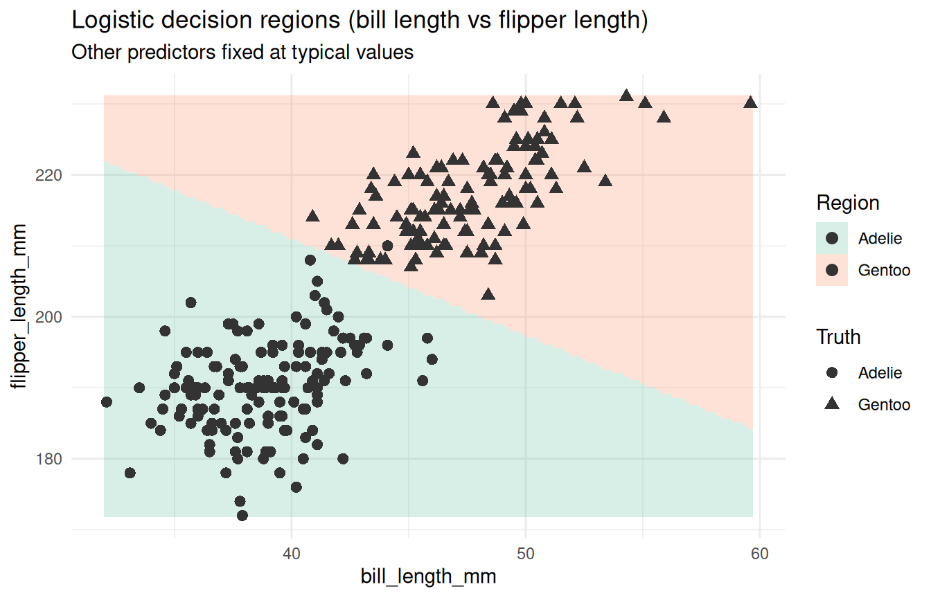
tidymodels pipeline include.