library(tidymodels)
library(palmerpenguins)
library(dplyr)
library(tidyr)
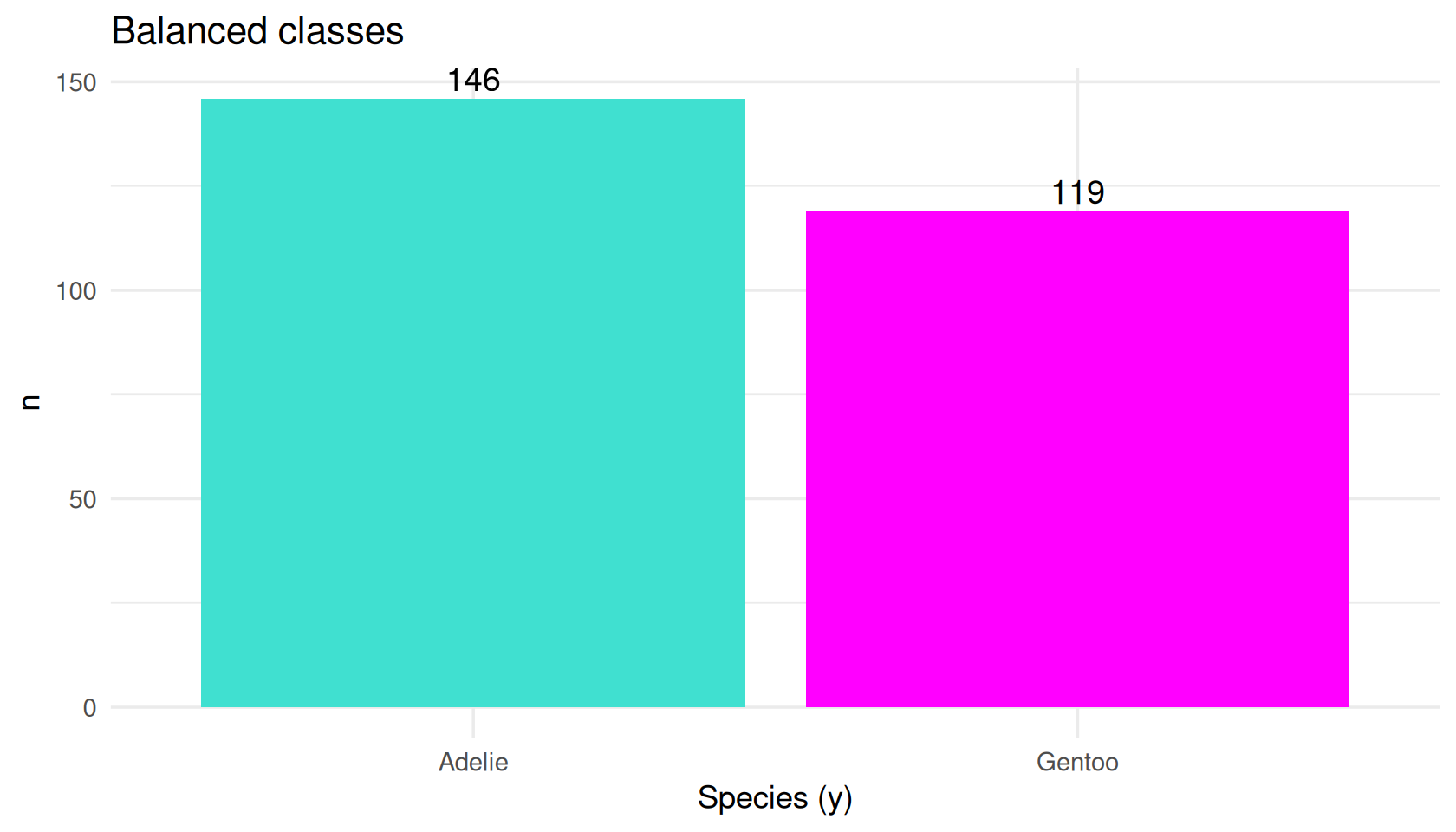
peng_cls <- palmerpenguins::penguins |>
dplyr::filter(species %in% c("Adelie", "Gentoo")) |>
dplyr::mutate(
y = factor(species, levels = c("Adelie", "Gentoo")),
year = as.numeric(year)
) |>
dplyr::select(-species, -flipper_length_mm, -body_mass_g) |>
tidyr::drop_na()Chapter 4: A reproducible modeling workflow
This chapter turns model building into a repeatable workflow. Instead of fitting, preprocessing, and scoring in disconnected scripts, we keep the full pipeline in one object so comparisons stay fair.
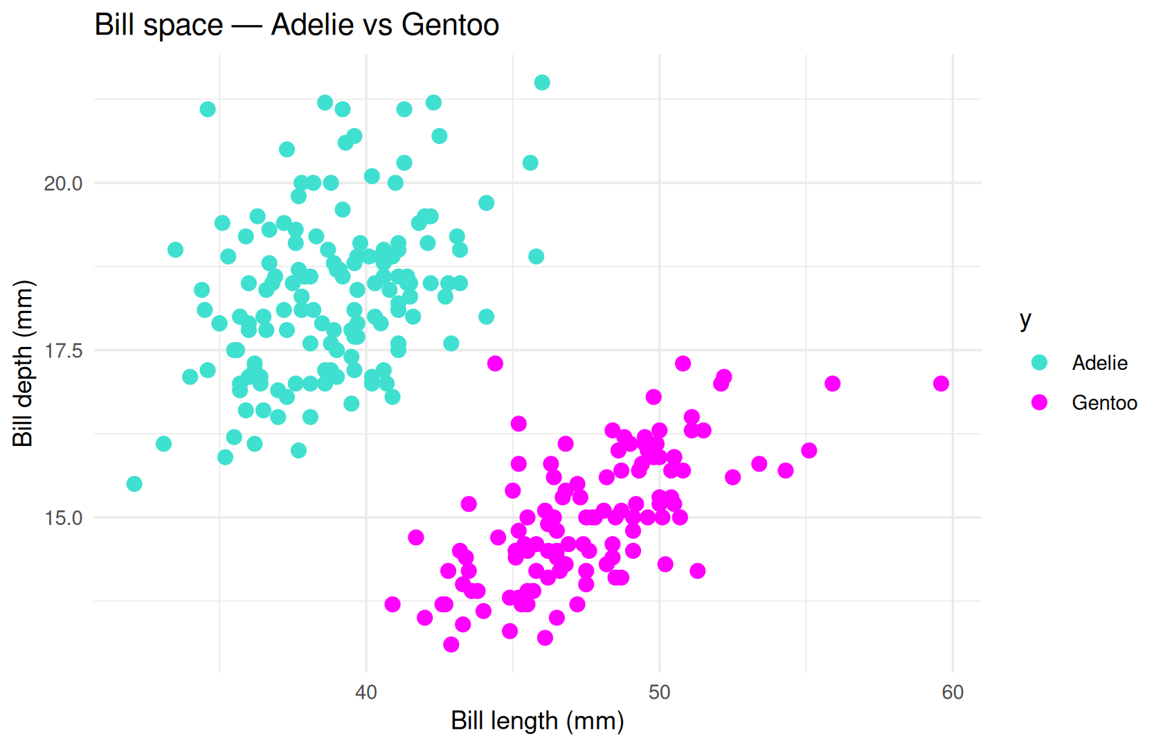
The teaching task is Adelie vs Gentoo classification. We use bill measures, island, sex, and year; we leave out flipper length and body mass so tuning remains informative rather than trivially high-scoring.
How to read this page
You already know lm and glm. Here we extend that mental model:
- A recipe is preprocessing.
- A model specification declares the learner.
- A workflow binds them.
tune_grid()explores settings with CV.
- First: one train/test split and
last_fit()to show the smallest honest flow.
- Then: the canonical Day 2 tuned tree include (shared with slides) for the full pattern.
← Reading companion · Back: Chapter 3 · Next: Chapter 5
First: one split, one model, no tuning (last_fit)
Day 2 (Tuesday) slides focus on cross-validation + tuning (faster to teach one rhythm in the room). If you want the smallest end-to-end tidymodels example first — hold out test rows, fit on training only, then score — work through this block.
Predictors (both sections): bill length & depth, island, sex, year — we drop flipper length and body mass so the tuned tree section below is not “everything wins at 99%.” The classification notebook still uses full morphology for classical glm / rpart plots.
Packages: tidymodels, palmerpenguins, dplyr, tidyr.
set.seed(11)
p_split <- initial_split(peng_cls, prop = 0.75, strata = y)
train <- training(p_split)
test <- testing(p_split)

count(train, y, name = "n_train")
# A tibble: 2 × 2
y n_train
<fct> <int>
1 Adelie 109
2 Gentoo 89count(test, y, name = "n_test")# A tibble: 2 × 2
y n_test
<fct> <int>
1 Adelie 37
2 Gentoo 30rec_tt <- recipe(y ~ ., data = train) |>
step_zv(all_predictors()) |>
step_dummy(all_nominal_predictors()) |>
step_normalize(all_numeric_predictors())mod_glm <- logistic_reg() |>
set_engine("glm") |>
set_mode("classification")
wf_tt <- workflow() |>
add_recipe(rec_tt) |>
add_model(mod_glm)fit_split <- last_fit(wf_tt, split = p_split, metrics = metric_set(accuracy, roc_auc))→ A | warning: glm.fit: algorithm did not converge→ B | warning: glm.fit: fitted probabilities numerically 0 or 1 occurredThere were issues with some computations A: x1 B: x1
There were issues with some computations A: x1 B: x1collect_metrics(fit_split)# A tibble: 2 × 4
.metric .estimator .estimate .config
<chr> <chr> <dbl> <chr>
1 accuracy binary 1 pre0_mod0_post0
2 roc_auc binary 1 pre0_mod0_post0collect_predictions(fit_split) |>
conf_mat(truth = y, estimate = .pred_class) Truth
Prediction Adelie Gentoo
Adelie 37 0
Gentoo 0 30When you continue to the canonical pipeline below, the include redefines peng_cls in a self-contained way (so slide chunks remain portable). The modeling grammar stays the same; only the resampling and tuning machinery becomes richer.
Canonical pipeline (Day 2 slides + tuning)
The next block is the same canonical walkthrough used in the Day 2 lecture deck. Keeping one shared include means the chapter and slides do not drift apart.
Palmer Penguins: one table, one model family (trees)
- Outcome
y: Adelie vs Gentoo (complete cases). - Predictors: bill length & depth, island, sex, year — no flipper or body mass (so
tree_depthandmin_nshow a real tuning tradeoff). - Today’s engine:
decision_tree()+rpartonly — forests and boosting come on Thursday.
The pipeline in principle
No code yet — the shape of every tidymodels project this week:
flowchart LR
  data[Raw table] --> recipe[recipe prep bake]
  recipe --> spec[parsnip spec]
  spec --> wf[workflow]
  folds[vfold_cv folds] --> tune[tune_grid]
  metrics[metric_set] --> tune
  wf --> tune
  tune --> best[select_best finalize]
  best --> fit[fit predict]
fit --> out[Plots and tables]- Recipe steps run inside each CV fold — never scale or encode on the full table before splitting (avoids leakage).
recipe/spec/workfloware blueprints; onlyfit(),fit_resamples(), andtune_grid()touch rows.- Today’s score: accuracy only; Thursday adds metrics for imbalanced data.
Five steps — what each one does
- Recipe — declare preprocessing steps (drop useless columns, dummy-code categories, scale numerics).
prep()learns rules on training rows;bake()applies them. - Spec — choose model type, engine, mode, and which arguments to tune. Still a blueprint — not fitted.
- Workflow — glue
recipe+specso onefit()runs preprocessing and training in the right order. - Metrics — define how to judge predictions (
accuracytoday). - Resample and tune — search hyperparameters on
vfold_cvfolds, pick the best, thenfitfor plots and interpretation.
Packages in the pipeline
| Package | Job |
|---|---|
rsample |
Training vs assessment rows (initial_split, vfold_cv) |
recipes |
Preprocessing checklist (dummy, scale, …) |
parsnip |
Model blueprint (decision_tree, set_engine("rpart")) |
workflows |
Glue recipe + model |
tune |
Search tree_depth and min_n |
yardstick |
Scores — accuracy only today; more metrics Thursday |
Step 1 — Preprocessing (recipe)
Turn raw columns into a model-ready table — in order, and only on training rows inside each fold.
Step 1 — Why a recipe?
- A recipe is a checklist of transforms applied before the model sees the data.
- Steps run top to bottom; order matters (e.g. dummy-code before scaling).
prep()learns parameters on training data;bake()applies them — aworkflow()does both automatically inside CV.
Start the recipe
rec <- recipe(y ~ ., data = peng_bal)
rec
recipe(y ~ ., data = peng_bal)—yis the outcome;.= all other columns are predictors.- Blueprint only — nothing transformed yet.
step_zv() — drop zero-variance columns
rec <- rec |>
  step_zv(all_predictors())
rec- Removes columns with one unique value (no predictive power; can break algorithms in small folds).
step_dummy() — encode categories
rec <- rec |>
  step_dummy(all_nominal_predictors())
recislandandsex→ numeric 0/1 columns forrpart.
step_normalize() — scale numeric predictors
rec <- rec |>
  step_normalize(all_numeric_predictors())
rec- Z-score each numeric column using training-fold rows only inside CV.
- Good habit before you swap in other model types later in the week.
rec_base <- rec
rec_base
prep() and bake() — learn rules, then apply
prep(recipe, training = train)estimates each step on training rows only.bake(prep, new_data = ...)applies those rules without re-learning (train, test, or new rows).- A
workflow()runsprep+bake+fitinside each CV fold automatically.
set.seed(2)
split_demo <- initial_split(peng_bal, prop = 0.75, strata = y)
train_demo <- training(split_demo)
test_demo <- testing(split_demo)

rec_prep <- prep(rec_base, training = train_demo)
bake_train <- bake(rec_prep, new_data = train_demo)
bake_test <- bake(rec_prep, new_data = test_demo)

dplyr::glimpse(bake_train)
Rows: 198
Columns: 7
$ bill_length_mm <dbl> -0.68460562, -0.60823834, -0.45550379, -1.14280927, -…
$ bill_depth_mm <dbl> 0.96969431, 0.30972785, 0.61432775, 1.27429421, 1.934…
$ year <dbl> -1.293173, -1.293173, -1.293173, -1.293173, -1.293173…
$ y <fct> Adelie, Adelie, Adelie, Adelie, Adelie, Adelie, Adeli…
$ island_Dream <dbl> -0.5175626, -0.5175626, -0.5175626, -0.5175626, -0.51…
$ island_Torgersen <dbl> 2.1159567, 2.1159567, 2.1159567, 2.1159567, 2.1159567…
$ sex_male <dbl> 0.9874465, -1.0075984, -1.0075984, -1.0075984, 0.9874…
NoteAfternoon lab (microbiome)
Same pattern on OTU counts — add step_mutate(..., log1p(.x)) on skewed abundances before step_zv.
Step 2 — Model blueprint (spec)
Choose the learner and its settings — still no fitting.
Step 2 — What is a spec?
parsnipstores the model family and hyperparameters in aspecobject.set_engine("rpart")picks the R implementation;set_mode("classification")matches a factor outcome.tune()marks arguments we will search later — the spec stays a blueprint untilfit().
Classification tree with rpart
tree_spec_demo <- decision_tree(tree_depth = 4, min_n = 10) |>
  set_engine("rpart") |>
  set_mode("classification")
tree_spec_demo
Decision Tree Model Specification (classification)
Main Arguments:
tree_depth = 4
min_n = 10
Computational engine: rpart decision_tree()— fixed parsnip function name.tree_depth,min_n— depth limit and minimum leaf size.set_engine("rpart")— same engine as the gene trees this morning.set_mode("classification")— factor outcomey.
Tuning knobs (tune())
tree_spec <- decision_tree(
  tree_depth = tune(),
  min_n = tune()
) |>
  set_engine("rpart") |>
  set_mode("classification")
tree_spec
Decision Tree Model Specification (classification)
Main Arguments:
tree_depth = tune()
min_n = tune()
Computational engine: rpart tune()marks argumentstune_grid()will search — we pick winners by cross-validated accuracy.
Parsnip: type → engine → mode
| Model type | Valid engines (examples) | Modes |
|---|---|---|
decision_tree() |
"rpart", "C5.0" |
classification, regression |
rand_forest() |
"ranger", "randomForest" |
classification, regression |
boost_tree() |
"xgboost", "lightgbm" |
classification, regression |
Thursday swaps spec — same recipe and workflow() pattern.
decision_tree() |>
set_engine("lm") |>
set_mode("classification")
# Error: 'lm' is not a valid engine for decision_tree()Step 3 — Workflow
Bundle preprocessing and model into one object.
Step 3 — Bundle recipe and model
workflow()combinesrec_baseandtree_specso you never preprocess the full table before splitting.add_recipe()+add_model()— one object to pass tofit(),tune_grid(), orfit_resamples().- Inside each resample, the workflow prep → bake → train on analysis rows only.
Step 3 — workflow() code
wf <- workflow() |>
add_recipe(rec_base) |>
add_model(tree_spec)
wf══ Workflow ════════════════════════════════════════════════════════════════════
Preprocessor: Recipe
Model: decision_tree()
── Preprocessor ────────────────────────────────────────────────────────────────
3 Recipe Steps
• step_zv()
• step_dummy()
• step_normalize()
── Model ───────────────────────────────────────────────────────────────────────
Decision Tree Model Specification (classification)

Main Arguments:
  tree_depth = tune()
  min_n = tune()

Computational engine: rpart Step 3 — One-shot fit (intuition)
fit(wf, data = peng_bal)on all rows is a quick way to see a decision boundary — not our final honest evaluation.- We use a fixed demo spec (
tree_spec_demo) so the plot is stable before tuning. - After tuning (Step 5), we refit on all rows for teaching plots; in a project, keep a locked test set.
Step 3 — Fit and boundary (code)
wf_demo <- workflow() |>
  add_recipe(rec_base) |>
  add_model(tree_spec_demo)
fit_demo <- fit(wf_demo, data = peng_bal)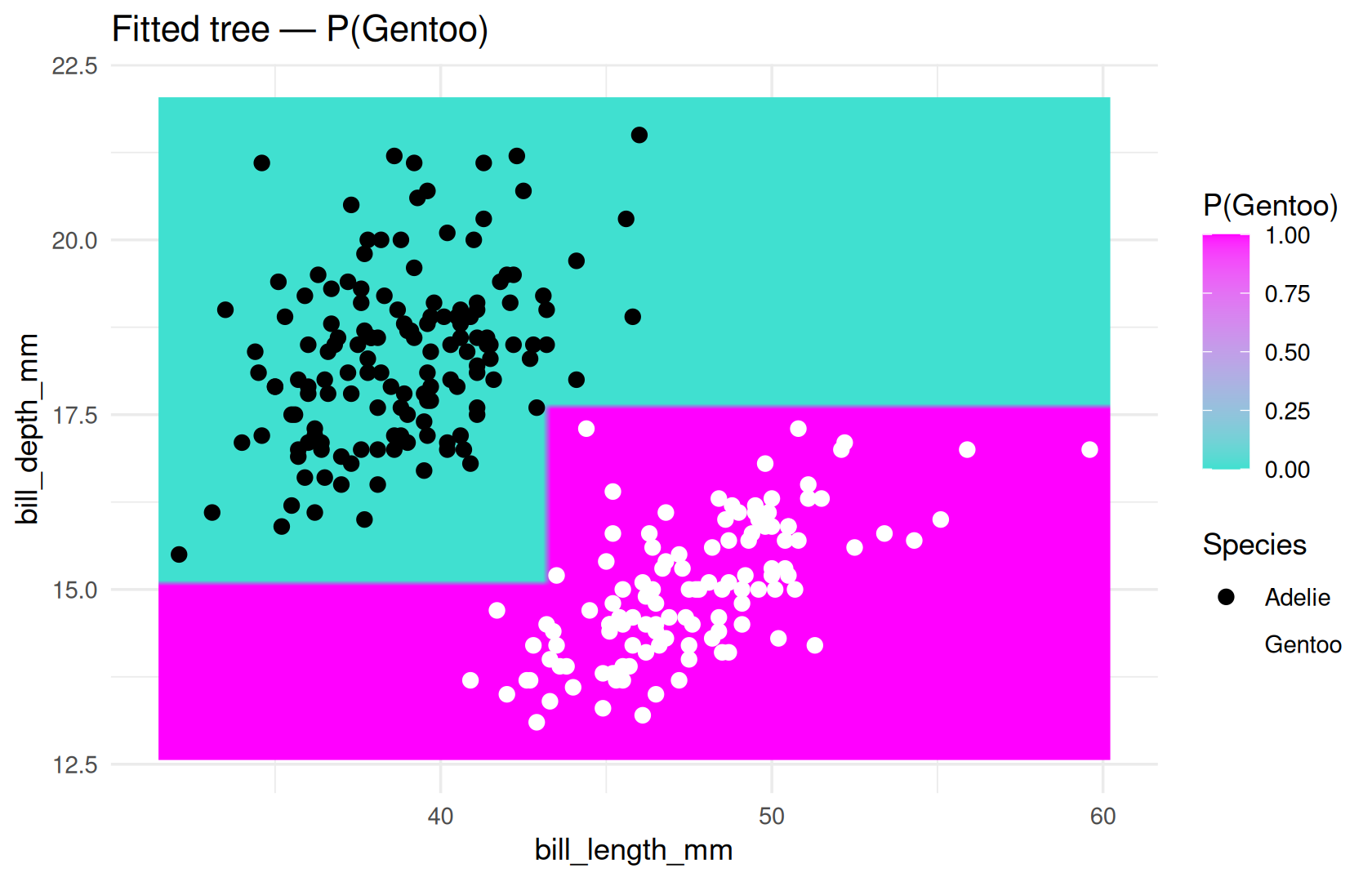
Step 4 — Metrics (accuracy today)
Decide how to score predictions before you tune.
Step 4 — Choose a metric before tuning
accuracy— fraction of correct class labels; fine when classes are balanced and errors cost the same.- Thursday: sensitivity, ROC-AUC, PR-AUC when the positive class is rare — accuracy can mislead.
metric_set(accuracy)bundles scorers fortune_grid()andfit_resamples().
Step 4 — metric_set code
metrics_day2A metric set, consisting of:
- `accuracy()`, a class metric | direction: maximizeStep 5 — Cross-validation and tuning
Search tree_depth and min_n on held-out folds, then finalize.
fit() vs fit_resamples() vs tune_grid()
| Function | Data splits | Parameter combinations |
|---|---|---|
fit() |
1 training set | 1 |
fit_resamples() |
Many folds/resamples | 1 |
tune_grid() |
Many folds/resamples | Many |
- Use
fit()when hyperparameters are already chosen. - Use
fit_resamples()to estimate CV performance for one fixed workflow. - Use
tune_grid()when you need to search over multiple hyperparameter values.
In this walkthrough: fit_demo (plot), rs_tree (CV, fixed params), tune_res (CV + search).
Step 5 — Search hyperparameters on folds
folds <- vfold_cv(..., strata = y)— each fold keeps both species represented.tune_grid(wf, resamples = folds, grid = ..., metrics = metrics_day2)tries many specs; preprocessing is refit inside each fold.- Grid spans stumps (depth 1, large
min_n) to more flexible trees.
Step 5 — tune_grid code
set.seed(2)
tune_res <- tune_grid(
wf,
resamples = folds,
grid = grid_regular(
tree_depth(range = c(1, 6)),
min_n(range = c(2, 50)),
levels = 4
),
metrics = metrics_day2
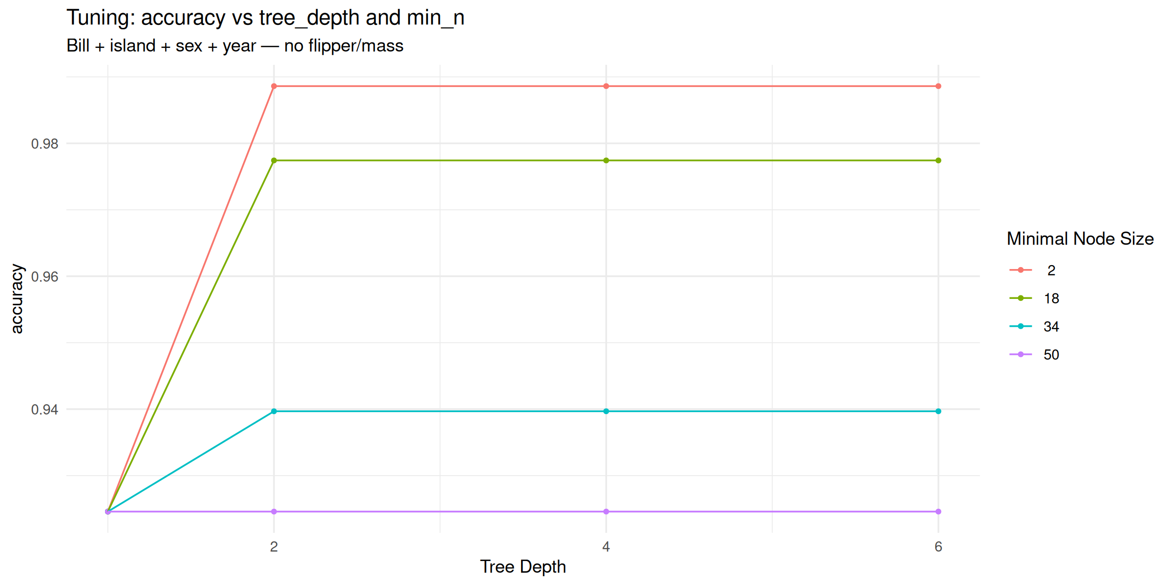
)Step 5 — Read the tuning plot
autoplot(tune_res)shows mean accuracy vstree_depthandmin_n.- Expect lower accuracy at
tree_depth = 1(stump) and with largemin_n(heavy pruning). - Pick a region that balances fit and simplicity before
select_best().
Step 5 — Tuning plot (code)
tune_res |>
  autoplot() +
  theme_minimal() +
  labs(
    title = "Tuning: accuracy vs tree_depth and min_n",
    subtitle = "Bill + island + sex + year — no flipper/mass"
  )
The honest evaluation workflow
You split your data into training and test sets, then use cross-validation on the training set to tune hyperparameters for each model and compute their average performance. For each model type, you select the best-performing hyperparameter combination based on CV results, and then compare these tuned models to choose the best overall model. Finally, you refit that selected model on the full training data and evaluate it once on the untouched test set to get an unbiased estimate of real-world performance.
| Stage | What happens | tidymodels tools (examples) |
|---|---|---|
| Hold out test data | Test rows stay unused until the very end | initial_split(), training(), testing() |
| Tune on training only | CV estimates average performance while searching hyperparameters | vfold_cv(), tune_grid(), select_best() |
| Compare learners | Same folds + recipe; pick the best model type after tuning each | fit_resamples(), collect_metrics() |
| Final report | Refit on all training rows; score once on test | last_fit() |
- Recipe steps (dummy, scale, impute, PCA, upsample, …) must be fit inside each CV fold on training rows only - otherwise information leaks from held-out data.
fit_resamples()(next) averages CV metrics for a workflow - quick comparisons when specs are fixed or already tuned.- Chapter 4 — train/test split walks through
last_fit()with a real train/test split.
Step 5 — Finalize and refit
select_best(tune_res, metric = "accuracy")— best hyperparameters from CV.finalize_workflow(wf, best)— plug tuned values into the blueprint.fit(final_wf, data = peng_cls)— one tree on all rows for plots;fit_resamples()reports honest CV performance.- In projects, use
last_fit()with a true test set instead of fitting on all rows for reporting.
Step 5 — Finalize and CV metrics (code)
best <- select_best(tune_res, metric = "accuracy")
final_wf <- finalize_workflow(wf, best)
final_fit <- fit(final_wf, data = peng_cls)
best
# A tibble: 1 × 3
tree_depth min_n .config
<int> <int> <chr>
1 2 2 pre0_mod05_post0set.seed(6)
wf_tree <- final_wf
rs_tree <- fit_resamples(wf_tree, folds, metrics = metrics_day2)
metrics_summary_table(rs_tree, "Tuned tree (5-fold CV)")# A tibble: 1 × 4
model .metric mean std_err
<chr> <chr> <dbl> <dbl>
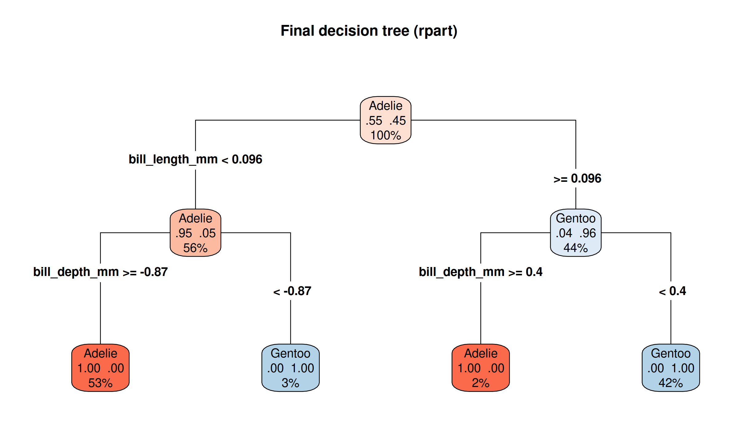
1 Tuned tree (5-fold CV) accuracy 0.989 0.00465Fitted tree structure
final_fit |>
  extract_fit_engine() |>
  rpart.plot(
    roundint = FALSE,
    type = 4,
    extra = 104,
    box.palette = "RdBu",
    main = "Final decision tree (rpart)"
  )
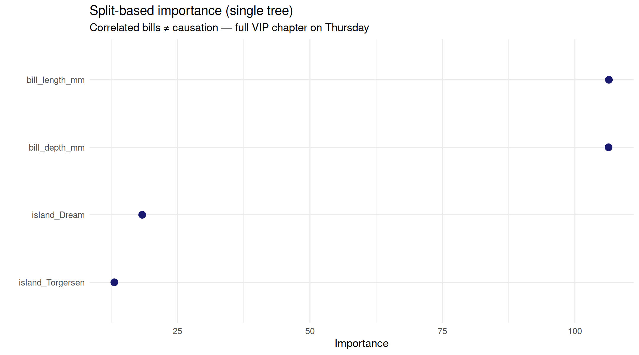
Variable importance (this tree)
final_fit |>
  extract_fit_parsnip() |>
  vip(geom = "point", aesthetics = list(color = "midnightblue", size = 3)) +
  theme_minimal() +
  labs(
    title = "Split-based importance (single tree)",
    subtitle = "Correlated bills ≠ causation — full VIP chapter on Thursday"
  )
Lecture: Day 2 (Tuesday) pipeline slides
Notebook: penguins-canonical-pipeline.Rmd
Next: Chapter 5 — Stronger learners, same discipline