data("penguins", package = "palmerpenguins")
pg <- penguins |>
  tidyr::drop_na()
nrow(pg)
[1] 333This notebook uses Palmer Penguins as a continuous outcome example: we predict body_mass_g from bill and flipper measurements (and simple factors).
It complements the synthetic gene linear / LASSO notebook (linear-regression-lasso.Rmd), where we know the ground truth. Here we work with real measurements and the usual messiness (correlation, nonlinear hints, missing values). Concepts for shrinkage sit in Module 02; this file is the long lab to run in the IDE.
data("penguins", package = "palmerpenguins")
pg <- penguins |>
tidyr::drop_na()
nrow(pg)[1] 333pg_num <- pg |>
select(bill_length_mm, bill_depth_mm, flipper_length_mm, body_mass_g)
cor_m <- cor(pg_num)
cor_df <- as.data.frame(as.table(cor_m)) |>
rename(v1 = Var1, v2 = Var2, r = Freq)
ggplot(cor_df, aes(v1, v2, fill = r)) +
geom_tile(color = "white") +
scale_fill_gradient2(low = "steelblue", mid = "white", high = "firebrick", midpoint = 0, limits = c(-1, 1)) +
theme_minimal() +
theme(axis.text.x = element_text(angle = 45, hjust = 1)) +
coord_fixed() +
labs(title = "Correlation among numeric penguin measurements")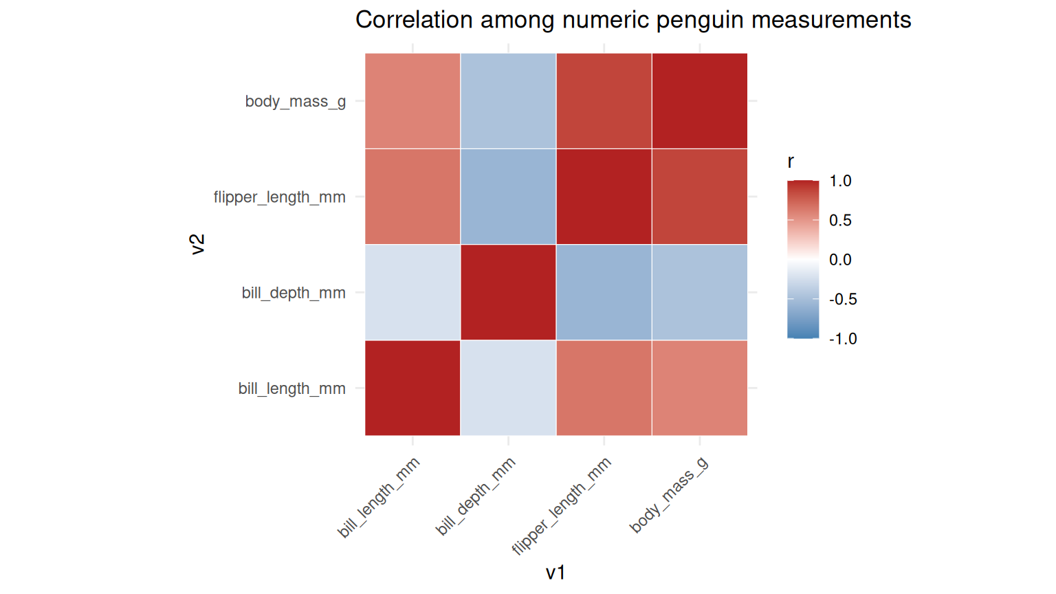
GGally::ggpairs(
  pg_num,
  upper = list(continuous = wrap("cor", size = 2.2)),
  aes(color = pg$species, alpha = 0.25)
) +
  theme(axis.text.x = element_text(angle = 45, hjust = 1))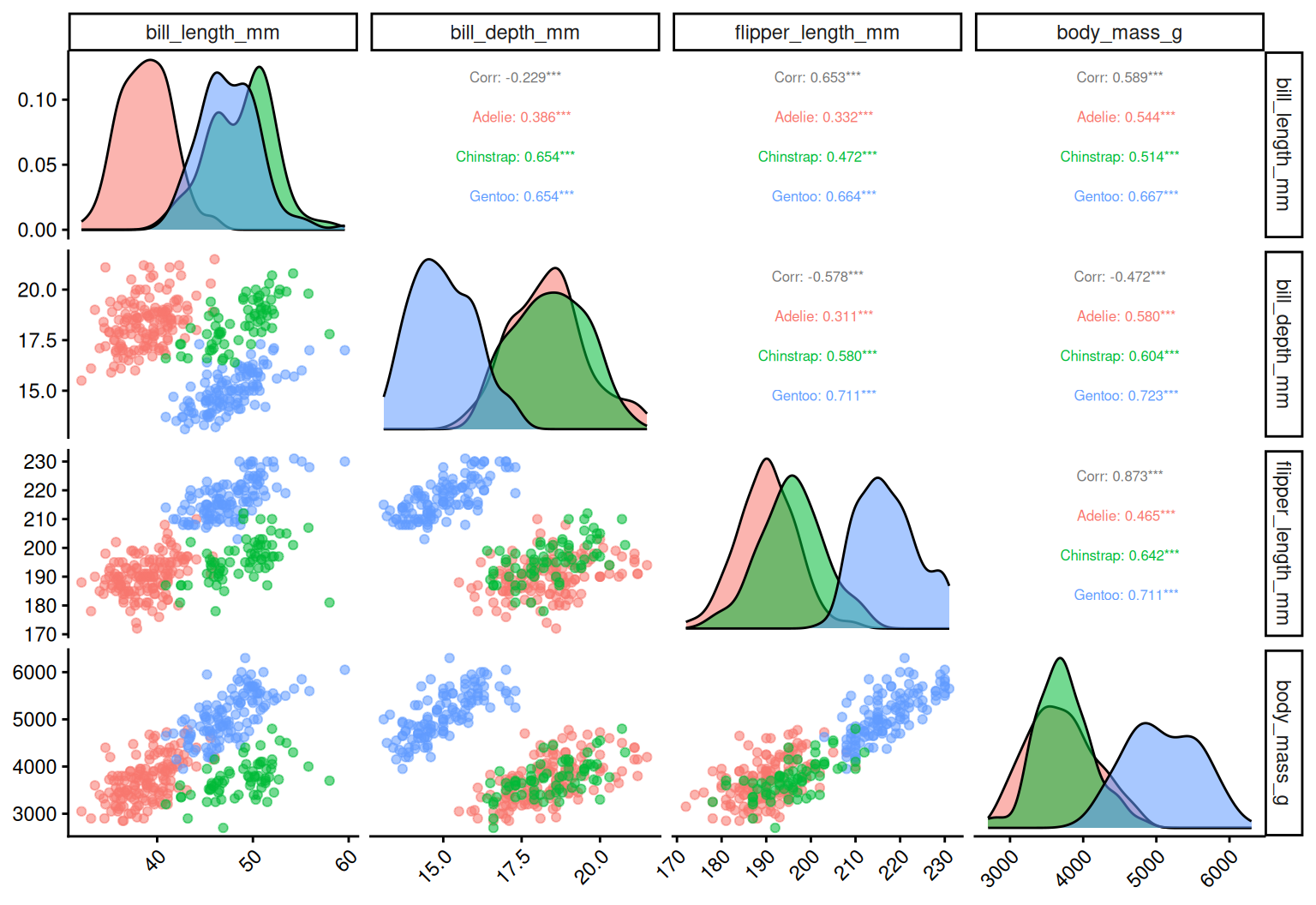
We model body_mass_g from morphometrics plus species, island, sex, and year (as numeric).
pred_df <- pg |>
  mutate(year = as.numeric(year)) |>
  select(body_mass_g, bill_length_mm, bill_depth_mm, flipper_length_mm, species, island, sex, year)

y <- pred_df$body_mass_g
X <- model.matrix(body_mass_g ~ ., data = pred_df)[, -1] # drop intercept column; dummy coding

set.seed(42)
split <- initial_split(pred_df, prop = 0.8)
train_df <- training(split)
test_df <- testing(split)
rm(split)

rec_scale <- recipe(body_mass_g ~ ., data = train_df) |>
  step_normalize(all_numeric_predictors())
prep_fit <- prep(rec_scale, train_df)
train_b <- bake(prep_fit, train_df)
test_b <- bake(prep_fit, test_df)

y_train <- train_b$body_mass_g
y_test <- test_b$body_mass_g
X_train_s <- model.matrix(body_mass_g ~ ., data = train_b)[, -1]
X_test_s <- model.matrix(body_mass_g ~ ., data = test_b)[, -1]cv_ridge <- cv.glmnet(X_train_s, y_train, alpha = 0)
cv_lasso <- cv.glmnet(X_train_s, y_train, alpha = 1)
par(mfrow = c(1, 2))
plot(cv_ridge, main = "Ridge CV")
plot(cv_lasso, main = "LASSO CV")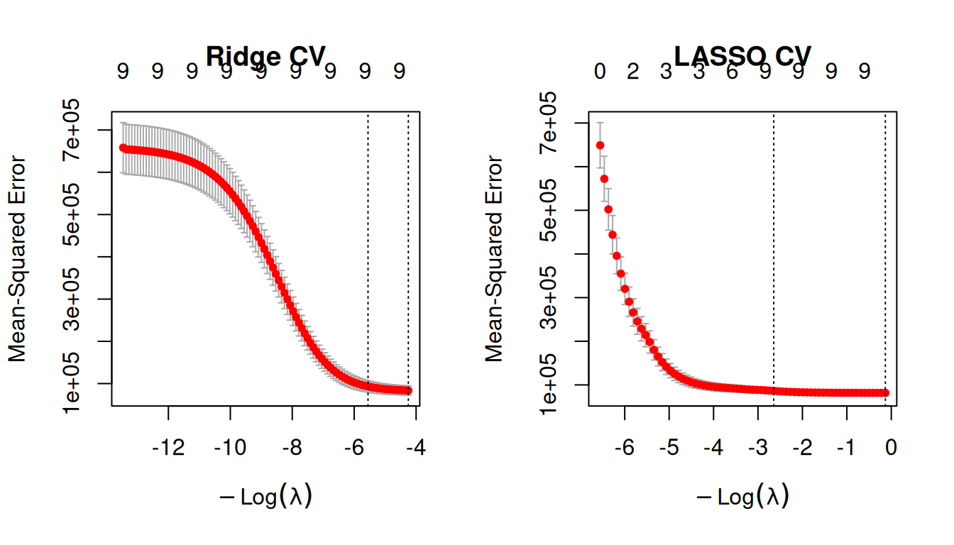
best_lam_ridge <- cv_ridge$lambda.min
best_lam_lasso <- cv_lasso$lambda.min
fit_ridge <- glmnet(X_train_s, y_train, alpha = 0, lambda = best_lam_ridge)
fit_lasso <- glmnet(X_train_s, y_train, alpha = 1, lambda = best_lam_lasso)

pred_ridge <- as.numeric(predict(fit_ridge, newx = X_test_s))
pred_lasso <- as.numeric(predict(fit_lasso, newx = X_test_s))

reg_metrics <- metric_set(rmse, rsq, mae)
tibble(truth = y_test, .pred = pred_ridge) |>
  reg_metrics(truth, .pred)
# A tibble: 3 × 3
.metric .estimator .estimate
<chr> <chr> <dbl>
1 rmse standard 313.
2 rsq standard 0.851
3 mae standard 254. tibble(truth = y_test, .pred = pred_lasso) |>
reg_metrics(truth, .pred)# A tibble: 3 × 3
.metric .estimator .estimate
<chr> <chr> <dbl>
1 rmse standard 310.
2 rsq standard 0.853
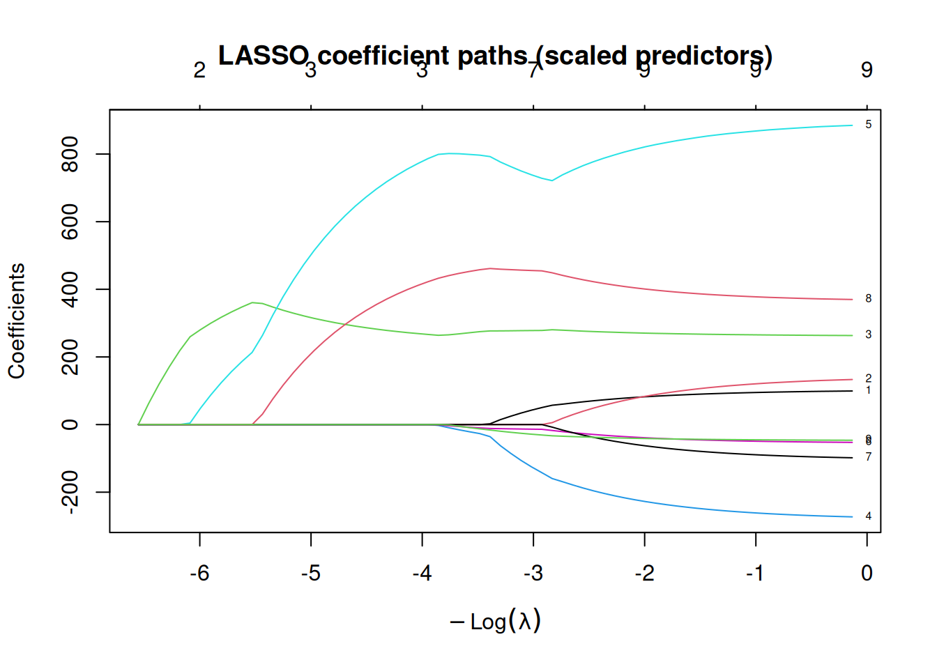
3 mae standard 249. fit_path <- glmnet(X_train_s, y_train, alpha = 1)
plot(fit_path, xvar = "lambda", label = TRUE, main = "LASSO coefficient paths (scaled predictors)")