peng <- penguins |>
  filter(species %in% c("Adelie", "Gentoo")) |>
  mutate(
    y = factor(species, levels = c("Adelie", "Gentoo")),
    year = as.numeric(year)
  ) |>
  select(-species, -flipper_length_mm, -body_mass_g) |>
  drop_na()

rec <- recipe(y ~ ., data = peng) |>
  step_zv(all_predictors()) |>
  step_dummy(all_nominal_predictors()) |>
  step_normalize(all_numeric_predictors())

folds <- vfold_cv(peng, v = 5, strata = y)
metrics <- metric_set(accuracy, kap, roc_auc)Palmer Penguins — canonical pipeline (three models, three metrics)
Overview
Minimal canonical tidymodels pipeline on Palmer Penguins (Adelie vs Gentoo):
- Recipe → preprocess inside resampling
- Three model specs → same folds, fair comparison
fit_resamples()→ accuracy, kappa, ROC AUC
- One summary figure (mean ± SE across folds)
Companion: Module 04 — canonical pipeline, Module 07, Module 08.
Data, recipe, and folds
Three models (fixed settings)
tree_spec <- decision_tree(tree_depth = 4, min_n = 10) |>
  set_engine("rpart") |>
  set_mode("classification")

glm_spec <- logistic_reg() |>
  set_engine("glm") |>
  set_mode("classification")

rf_spec <- rand_forest(mtry = 4, trees = 300, min_n = 2) |>
  set_engine("ranger") |>
  set_mode("classification")

workflows <- list(
  decision_tree = workflow() |> add_recipe(rec) |> add_model(tree_spec),
  logistic_glm = workflow() |> add_recipe(rec) |> add_model(glm_spec),
  random_forest = workflow() |> add_recipe(rec) |> add_model(rf_spec)
)
Cross-validation (fit_resamples)
set.seed(7)
cv_results <- workflows |>
  imap(\(wf, name) fit_resamples(wf, folds, metrics = metrics)) |>
  set_names(names(workflows))
Metrics table
cmp <- imap_dfr(
  cv_results,
  \(rs, name) collect_metrics(rs) |> mutate(model = name)
)

cmp |>
  select(model, .metric, mean, std_err) |>
  mutate(
    mean = round(mean, 3),
    std_err = round(std_err, 3)
  ) |>
  arrange(.metric, desc(mean)) |>
knitr::kable(col.names = c("Model", "Metric", "Mean", "Std err"))| Model | Metric | Mean | Std err |
|---|---|---|---|
| logistic_glm | accuracy | 1.000 | 0.000 |
| random_forest | accuracy | 1.000 | 0.000 |
| decision_tree | accuracy | 0.993 | 0.005 |
| logistic_glm | kap | 1.000 | 0.000 |
| random_forest | kap | 1.000 | 0.000 |
| decision_tree | kap | 0.985 | 0.009 |
| logistic_glm | roc_auc | 1.000 | 0.000 |
| random_forest | roc_auc | 1.000 | 0.000 |
| decision_tree | roc_auc | 0.993 | 0.004 |
Performance summary (final figure)
Same recipe and folds for every model — differences reflect model family only.
plot_df <- cmp |>
  mutate(
    model = recode(
      model,
      decision_tree = "Decision tree",
      logistic_glm = "Logistic regression",
      random_forest = "Random forest"
    ),
    metric = recode(
      .metric,
      accuracy = "Accuracy",
      kap = "Kappa",
      roc_auc = "ROC AUC"
    )
  )

ggplot(plot_df, aes(model, mean, fill = model)) +
  geom_col(show.legend = FALSE, width = 0.72) +
  geom_errorbar(
    aes(ymin = mean - std_err, ymax = mean + std_err),
    width = 0.18,
    linewidth = 0.5
  ) +
  facet_wrap(~metric, scales = "free_y", ncol = 3) +
  coord_flip() +
  scale_fill_brewer(palette = "Set2") +
  labs(
    title = "Model comparison (5-fold CV, same recipe)",
    subtitle = "Bars = mean across folds; error bars = standard error",
    x = NULL,
    y = "Score (higher is better)"
  ) +
  theme_minimal(base_size = 13) +
  theme(strip.text = element_text(face = "bold"))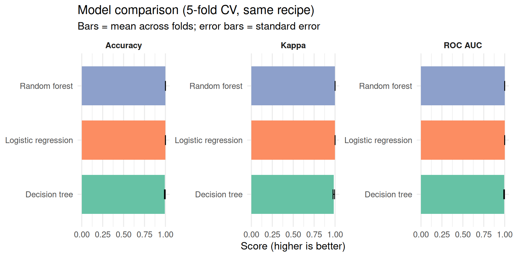
Takeaway: pick the metric that matches your goal (e.g. ROC AUC for ranking, kappa when classes are imbalanced), then compare models on that score — small gaps within the error bars are often noise on this (n).