---
title: "Palmer Penguins — three-species classification"
author: "Aparna Pandey and Stephan Peischl"
format:
html:
toc: true
code-tools: true
engine: knitr
---
```{r setup, include=FALSE}
knitr::opts_chunk$set(echo = TRUE, message = FALSE, warning = FALSE)
library(palmerpenguins)
library(dplyr)
library(ggplot2)
library(GGally)
library(nnet)
library(rpart)
library(rpart.plot)
library(tidymodels)
library(tidyr)
theme_set(theme_classic())
```
# Overview
Here we treat **`species`** as a **three-level** outcome (Adelie, Chinstrap, Gentoo) using **multinomial logistic regression** (`nnet::multinom`) and a **multiclass classification tree** (`rpart`). This complements the **binary** Adelie-vs-Gentoo notebook (`penguins-classification.Rmd`). For **metrics and multiclass intuition** on the site, see [Module 06](../modules/module-06-evaluation-and-interpretability.qmd).
See **[Palmer Penguins data card](../data/cards/palmer-penguins.qmd)**.
## Prepare data
```{r}
data("penguins", package = "palmerpenguins")
pg <- penguins |>
  tidyr::drop_na(species, bill_length_mm, bill_depth_mm, flipper_length_mm, body_mass_g, island, sex, year) |>
  mutate(
    species = droplevels(species),
    year = as.numeric(year)
  )

table(pg$species)
nrow(pg)
```
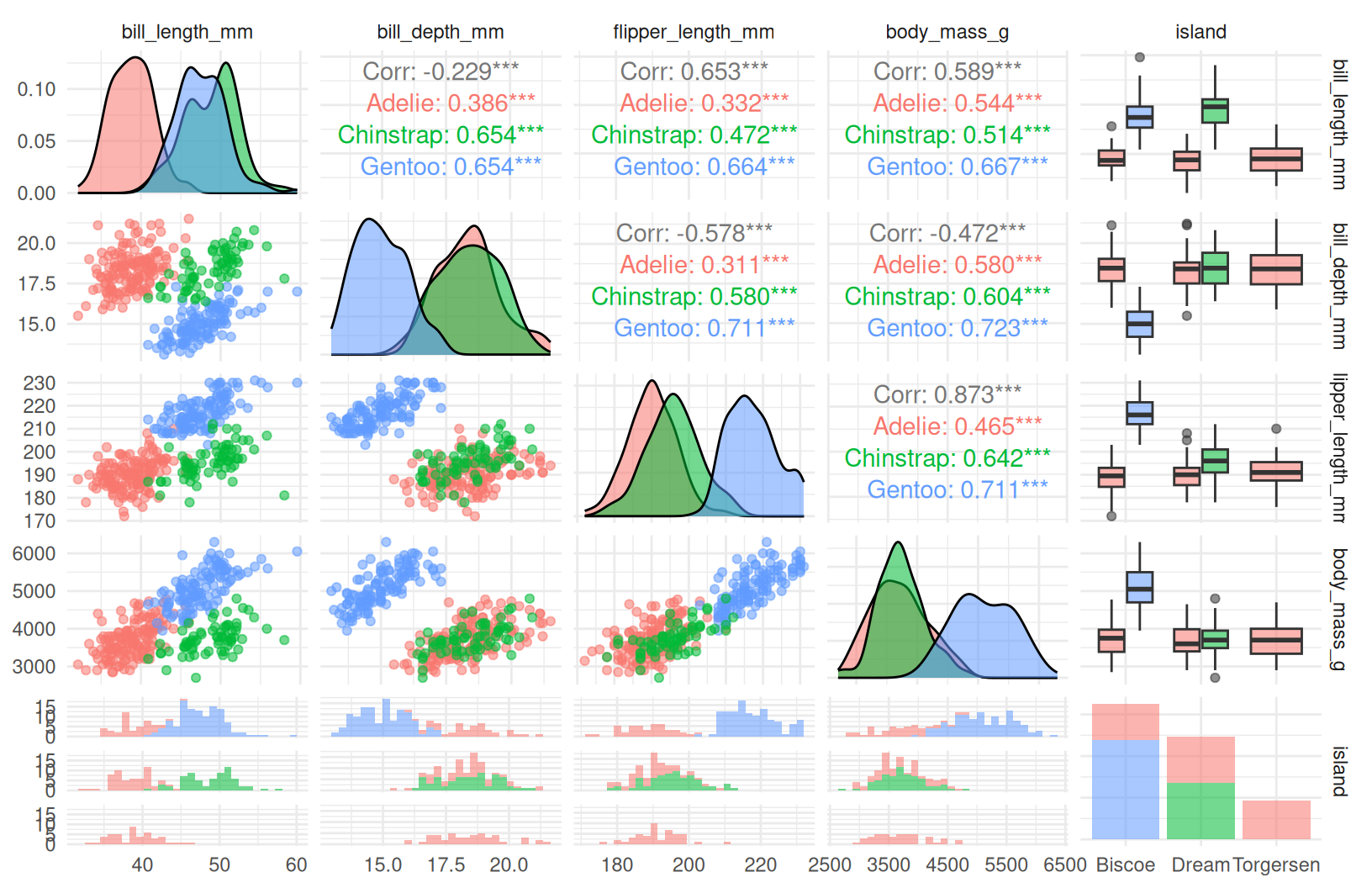
## Pair plot (measurements + island, coloured by species)
```{r fig.width=8.5, fig.height=5.5}
GGally::ggpairs(
  pg,
  columns = c("bill_length_mm", "bill_depth_mm", "flipper_length_mm", "body_mass_g", "island"),
  aes(color = species, alpha = 0.25)
) +
  theme_minimal()
```
## Train / test split (stratified on `species`)
```{r}
set.seed(24)
split <- initial_split(pg, prop = 0.75, strata = species)
train <- training(split)
test <- testing(split)
```
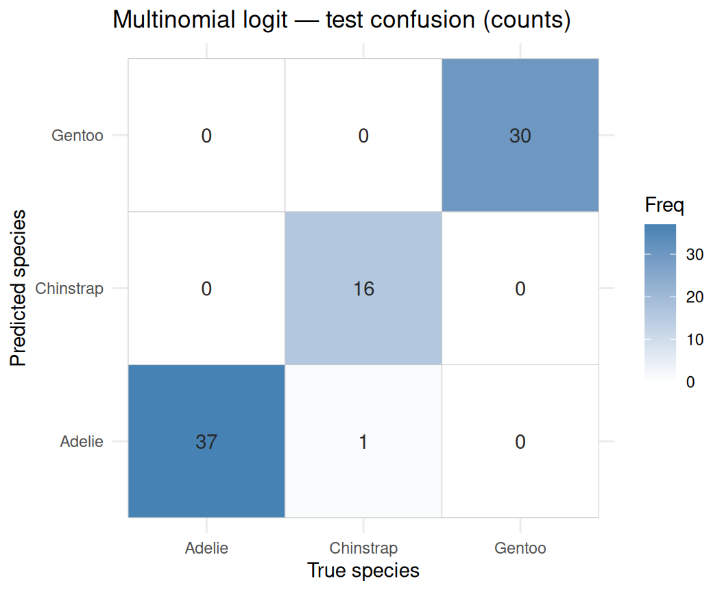
## Multinomial logistic regression
```{r}
set.seed(1)
multi_fit <- nnet::multinom(
  species ~ bill_length_mm + bill_depth_mm + flipper_length_mm + body_mass_g + island + sex + year,
  data = train,
  trace = FALSE,
  MaxNWts = 5000
)
summary(multi_fit)
```
```{r}
pred_multi <- predict(multi_fit, newdata = test)
tibble(truth = test$species, .pred_class = pred_multi) |>
  conf_mat(truth = truth, estimate = .pred_class)
```
```{r fig.width=5.5, fig.height=4.5}
cm_obj <- conf_mat(
  tibble(truth = test$species, .pred_class = pred_multi),
  truth = truth,
  estimate = .pred_class
)
cm <- as.data.frame.table(cm_obj$table, stringsAsFactors = FALSE) |>
  dplyr::rename(Reference = Truth)
ggplot(cm, aes(Reference, Prediction, fill = Freq)) +
  geom_tile(color = "gray80") +
  geom_text(aes(label = Freq), color = "gray15") +
  scale_fill_gradient(low = "white", high = "steelblue") +
  theme_minimal() +
  labs(
    title = "Multinomial logit — test confusion (counts)",
    x = "True species", y = "Predicted species"
  )
```
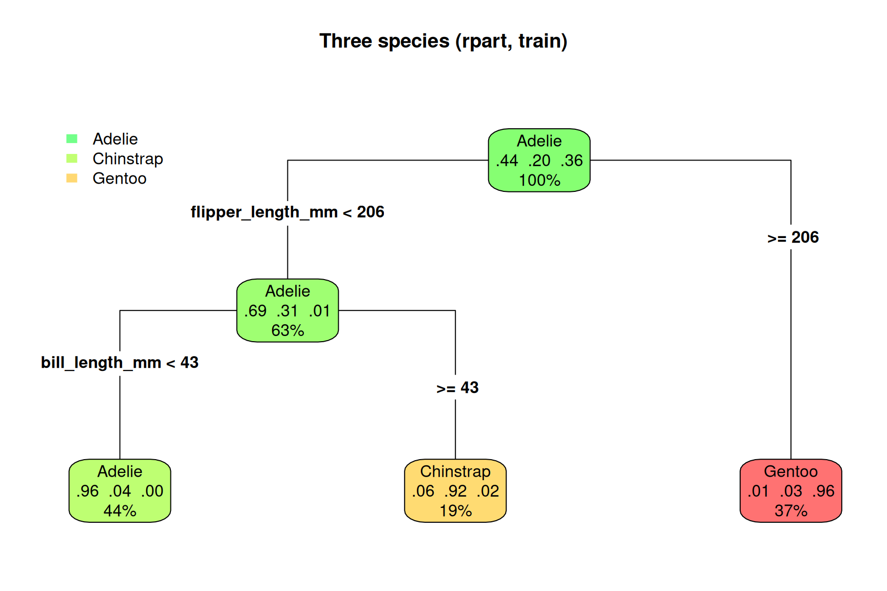
## Multiclass tree
```{r fig.width=9, fig.height=6}
tree_fit <- rpart(
  species ~ bill_length_mm + bill_depth_mm + flipper_length_mm + body_mass_g + island + sex + year,
  data = train,
  method = "class"
)
rpart.plot(tree_fit, type = 4, extra = 104, box.palette = "GnYlRd", main = "Three species (rpart, train)")
```
```{r}
pred_t <- predict(tree_fit, test, type = "class") |> factor(levels = levels(test$species))
tibble(truth = test$species, .pred_class = pred_t) |>
  conf_mat(truth = truth, estimate = .pred_class)
```
## Takeaways
- **Chinstrap** is often the hardest class (smaller *n*, overlap in measurement space) — inspect **per-class** metrics, not only overall accuracy.
- Multiclass **ROC** and **one-vs-rest** calibration are natural Thursday extensions; here we stay with **confusion matrices** + trees for clarity.
- Compare with the **binary** pipeline in `_includes/day02-tidymodels-walkthrough.qmd` (Adelie vs Gentoo slice).