Palmer Penguins — PCA walkthrough

Overview

Self-contained PCA example on Palmer Penguins.

• Data: Adelie vs Gentoo slice
• PCA: centered/scaled numeric predictors and two components
• One model type: boosted tree (xgboost) with and without PCA

Related: Day 4 PCA block

Load data

peng_pca <- palmerpenguins::penguins |>
  filter(species %in% c("Adelie", "Gentoo")) |>
  mutate(
    y = factor(species, levels = c("Adelie", "Gentoo")),
    year = as.numeric(year)
  ) |>
  select(-species) |>
  tidyr::drop_na()

peng_pca |>
  count(y) |>
  knitr::kable(col.names = c("Species", "n"))

Species	n
Adelie	146
Gentoo	119

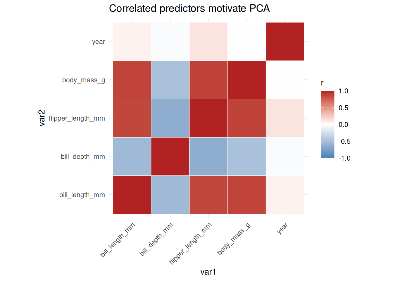
Correlation motivation

num_cols <- c("bill_length_mm", "bill_depth_mm", "flipper_length_mm", "body_mass_g", "year")
cor_df <- as.data.frame(as.table(cor(peng_pca[, num_cols]))) |>
  rename(var1 = Var1, var2 = Var2, r = Freq)

ggplot(cor_df, aes(var1, var2, fill = r)) +
  geom_tile(color = "white") +
  scale_fill_gradient2(low = "steelblue", mid = "white", high = "firebrick", midpoint = 0, limits = c(-1, 1)) +
  coord_fixed() +
  theme_minimal() +
  theme(axis.text.x = element_text(angle = 45, hjust = 1)) +
  labs(title = "Correlated predictors motivate PCA", fill = "r")

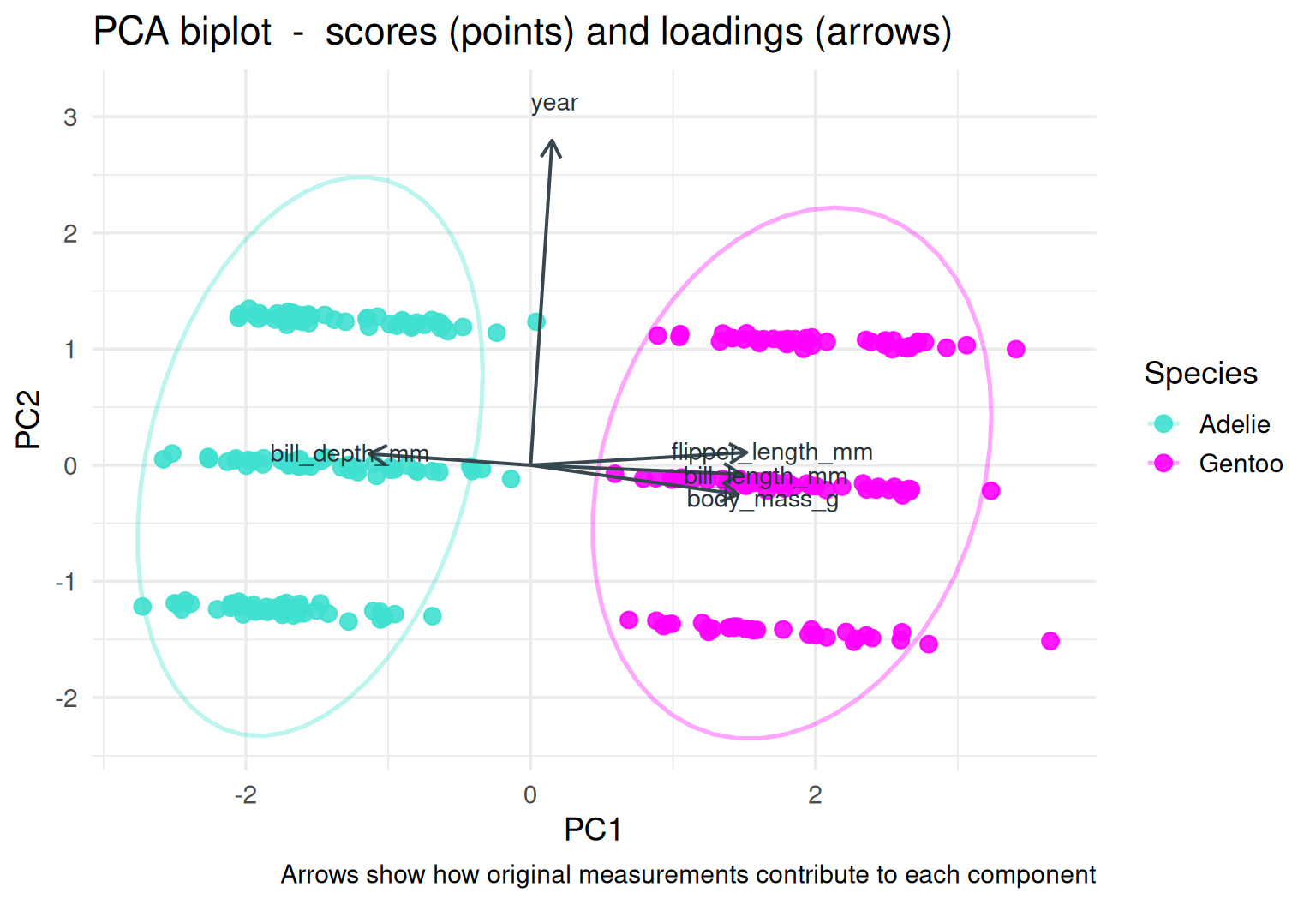
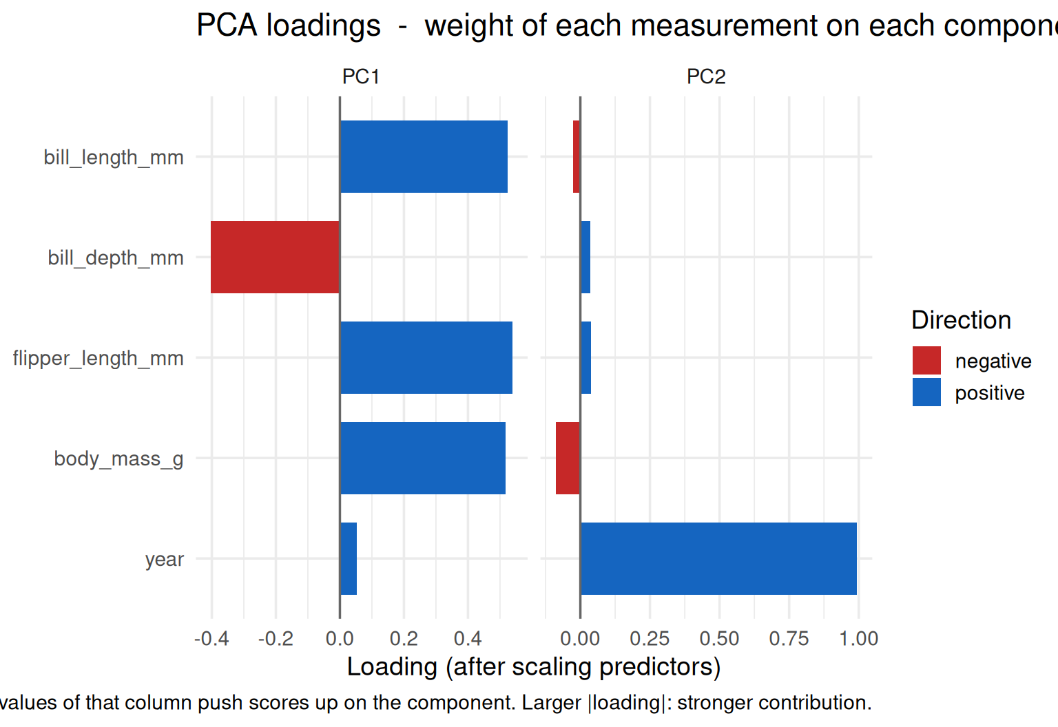
PCA geometry and loadings

plot_pca_biplot(peng_pca, num_cols = num_cols, y_col = "y")

plot_pca_loadings_bars(peng_pca, num_cols = num_cols)

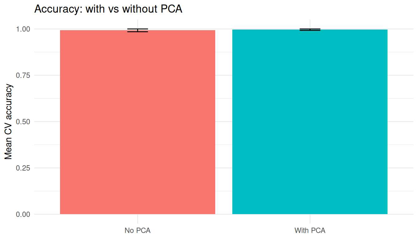
Minimal model usage (with vs without PCA)

set.seed(8)
folds <- vfold_cv(peng_pca, v = 5, strata = y)
metrics_acc <- metric_set(accuracy)

xgb_spec <- boost_tree(trees = 100, tree_depth = 3, learn_rate = 0.05) |>
  set_engine("xgboost") |>
  set_mode("classification")

rec_pca <- recipe(y ~ ., data = peng_pca) |>
  step_zv(all_predictors()) |>
  step_dummy(all_nominal_predictors()) |>
  step_normalize(all_numeric_predictors()) |>
  step_pca(all_numeric_predictors(), num_comp = 2)

rec_no_pca <- recipe(y ~ ., data = peng_pca) |>
  step_zv(all_predictors()) |>
  step_dummy(all_nominal_predictors()) |>
  step_normalize(all_numeric_predictors())

wf_pca <- workflow() |> add_recipe(rec_pca) |> add_model(xgb_spec)
wf_no_pca <- workflow() |> add_recipe(rec_no_pca) |> add_model(xgb_spec)

rs_pca <- fit_resamples(wf_pca, folds, metrics = metrics_acc)
rs_no <- fit_resamples(wf_no_pca, folds, metrics = metrics_acc)

bind_rows(
  collect_metrics(rs_pca) |> mutate(model = "XGB + PCA (2 comp.)"),
  collect_metrics(rs_no) |> mutate(model = "XGB without PCA")
) |>
  filter(.metric == "accuracy") |>
  select(model, mean, std_err) |>
  knitr::kable(caption = "5-fold CV accuracy")

5-fold CV accuracy

model	mean	std_err
XGB + PCA (2 comp.)	0.9961538	0.0038462
XGB without PCA	0.9924528	0.0075472

bind_rows(
  collect_metrics(rs_pca) |> mutate(model = "With PCA"),
  collect_metrics(rs_no) |> mutate(model = "No PCA")
) |>
  filter(.metric == "accuracy") |>
  ggplot(aes(model, mean, fill = model)) +
  geom_col(show.legend = FALSE) +
  geom_errorbar(aes(ymin = mean - std_err, ymax = mean + std_err), width = 0.12) +
  theme_minimal() +
  labs(title = "Accuracy: with vs without PCA", x = NULL, y = "Mean CV accuracy")

Takeaway

PCA can reduce correlated dimensions, but component-based models are often harder to explain biologically than models on original measurements.