library(tidymodels)
library(palmerpenguins)
library(dplyr)
library(tidyr)

peng_cls <- palmerpenguins::penguins |>
  dplyr::filter(species %in% c("Adelie", "Gentoo")) |>
  dplyr::mutate(
    y = factor(species, levels = c("Adelie", "Gentoo")),
    year = as.numeric(year)
  ) |>
  dplyr::select(-species, -flipper_length_mm, -body_mass_g) |>
  tidyr::drop_na()

rec <- recipe(y ~ ., data = peng_cls) |>
  step_zv(all_predictors()) |>
  step_dummy(all_nominal_predictors()) |>
  step_normalize(all_numeric_predictors())

mod_spec <- decision_tree(
  tree_depth = tune(),
  min_n = tune()
) |>
  set_engine("rpart") |>
  set_mode("classification")

wf <- workflow() |>
  add_recipe(rec) |>
  add_model(mod_spec)

folds <- vfold_cv(peng_cls, v = 5, strata = y)

metrics_all <- metric_set(accuracy, kap, roc_auc)Chapter 7: Choosing what to optimize (accuracy, kappa, ROC AUC)
ImportantExtension chapter — not the Tuesday lecture default
This chapter asks a practical question: if you keep data, folds, and model family fixed, what changes when you optimize for a different metric?
Build on Module 04 (train/test + glm) and Module 04 — canonical pipeline (recipe + tree + tune_grid from the shared include). Here we keep cross-validated tuning on the full peng_cls table — same Adelie vs Gentoo columns as Day 2 (Tuesday) slides (bill + island + sex + year; no flipper or body mass). Teaching default: tune on all rows; in a paper you would nest tuning inside training after a test lockbox.
Packages: same as Module 04 (tidymodels, palmerpenguins, dplyr, tidyr).
← Chapter 4 (train/test beat) · Reading companion · Next: Chapter 8 →
One grid, three metrics
kap is Cohen’s kappa: it subtracts what you would expect from guessing the majority class, so it is often more informative than raw accuracy when class counts differ.
set.seed(42)
tune_res <- tune_grid(
  wf,
  resamples = folds,
  grid = grid_regular(
    tree_depth(range = c(2, 6)),
    min_n(range = c(2, 20)),
    levels = 3
  ),
  metrics = metrics_all
)
What cross-validation reported (mean per setting)
collect_metrics(tune_res) |>
  dplyr::filter(.metric %in% c("accuracy", "kap", "roc_auc")) |>
  dplyr::arrange(.metric, desc(mean))
# A tibble: 27 × 8
tree_depth min_n .metric .estimator mean n std_err .config
<int> <int> <chr> <chr> <dbl> <int> <dbl> <chr>
1 2 2 accuracy binary 0.996 5 0.00377 pre0_mod1_post0
2 4 2 accuracy binary 0.996 5 0.00377 pre0_mod4_post0
3 6 2 accuracy binary 0.996 5 0.00377 pre0_mod7_post0
4 2 11 accuracy binary 0.992 5 0.00755 pre0_mod2_post0
5 4 11 accuracy binary 0.992 5 0.00755 pre0_mod5_post0
6 6 11 accuracy binary 0.992 5 0.00755 pre0_mod8_post0
7 2 20 accuracy binary 0.977 5 0.0110 pre0_mod3_post0
8 4 20 accuracy binary 0.977 5 0.0110 pre0_mod6_post0
9 6 20 accuracy binary 0.977 5 0.0110 pre0_mod9_post0
10 2 2 kap binary 0.992 5 0.00759 pre0_mod1_post0
# ℹ 17 more rowsSame tuning run — three different “winners”
best_acc <- select_best(tune_res, metric = "accuracy")
best_kap <- select_best(tune_res, metric = "kap")
best_auc <- select_best(tune_res, metric = "roc_auc")

best_acc
# A tibble: 1 × 3
tree_depth min_n .config
<int> <int> <chr>
1 2 2 pre0_mod1_post0best_kap# A tibble: 1 × 3
tree_depth min_n .config
<int> <int> <chr>
1 2 2 pre0_mod1_post0best_auc# A tibble: 1 × 3
tree_depth min_n .config
<int> <int> <chr>
1 2 2 pre0_mod1_post0If the three tibbles differ, that is the lesson: the metric is part of the scientific question, not an afterthought.
Optional — tuning surface (one panel per metric)
autoplot() draws one metric at a time here; re-run the chunk with metric = "accuracy" or "kap" to compare shapes.
autoplot(tune_res, metric = "roc_auc")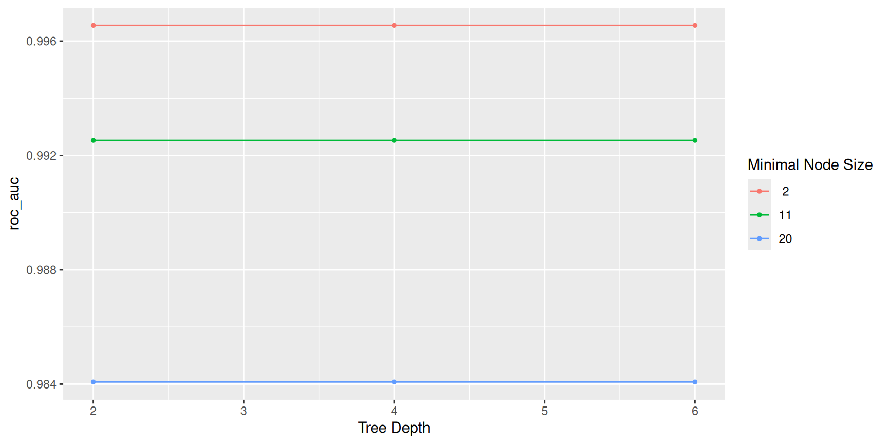
Takeaways
- You can commit to several metrics before tuning, then declare which one picks hyperparameters for this exercise (or use a rule: e.g. maximize kappa subject to sensitivity ≥ some floor).
- ROC AUC ranks risk; accuracy counts hard calls; kappa penalizes “always guess the common species” shortcuts.
- Chapter 8 holds the metric fixed and swaps model families.
Chapter links
- Concepts: Chapter 6 — Scores that match the question
- Day 4 (Thursday) slides: Metrics toolbox