# Load required libraries
library(yardstick)
library(rpart)
library(ggplot2)
library(rlang)
library(GGally)

# Set seed for reproducibility
set.seed(123)

# Number of samples
n <- 200

# Number of genes (features)
p <- 10

# Generate gene names
gene_names <- paste0("Gene", 1:p)

# Generate gene expression levels
genes_data <- data.frame(matrix(rnorm(n * p), nrow = n))
colnames(genes_data) <- gene_names

# True coefficients representing gene influence on disease presence
true_coefficients <- c(0.5, rep(0, 1), 0.8, -0.3, rep(0, p - 3))

# Generate disease trait presence based on gene expression levels
disease_presence <- ifelse(0.5 * genes_data$Gene1 + 0.8 * genes_data$Gene3 - 0.3 * genes_data$Gene4 - genes_data$Gene1*genes_data$Gene3 * 2 + rnorm(n, sd=0.5) > 0, 1, 0)

# Convert disease_presence to a factor with consistent levels
disease_presence <- factor(disease_presence, levels = c(0, 1), labels = c("Absent", "Present"))

# Combine gene expression and disease presence into a single data frame
bio_data <- data.frame(genes_data, disease_presence)Gene expression and Disease
Introduction
In this analysis, we simulate a biological dataset where gene expression levels influence the presence or absence of a disease trait. We generate synthetic gene expression data, create a response variable (disease_presence), and fit logistic regression and decision tree models. Finally, we evaluate and visualize the models.
Concept companions (short reads on the site): Module 01 — Foundations (splits and generalization) and Module 03 — Trees — this file is the long gene lab with all simulation and plots.
Summary of the Script
Dataset Generation:
- Number of Samples (n): 200
- Number of Features (p): 10 genes (named Gene1 to Gene10)
- Gene Expression Data: Simulated as normally distributed random values.
- Causal Genes:
- Gene1: Positive effect with a coefficient of 0.5, plus interaction with Gene3.
- Gene3: Positive effect with a coefficient of 0.8, plus interaction with Gene1.
- Gene4: Negative effect with a coefficient of -0.3.
- Response Variable (disease_presence): Binary (indicating the presence or absence of a disease trait) generated based on a linear combination of Gene1, Gene3, and Gene4 with some added noise.
Modeling:
- Logistic Regression: A generalized linear model (glm) with a binomial family was used to model the binary response variable (disease_presence).
- Decision Tree (rpart): A recursive partitioning tree was used to classify the binary response variable.
Visualization:
Pair Plot: Shows relationships among Gene1 to Gene4, colored by the response variable (disease_presence).
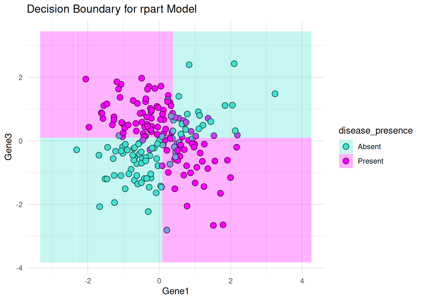
Decision Boundaries: Plots decision boundaries for logistic regression and the rpart model using Gene1 and Gene3 as features.
Data Generation
We simulate gene expression data for 200 samples and 10 genes. Gene1, Gene3, and Gene4 are causal genes influencing disease presence.
Visualizations
# Pair Plot of some features colored by disease presence
pair_plot <- ggpairs(bio_data, columns = 1:5, aes(color = disease_presence)) +
  theme_minimal()
print(pair_plot)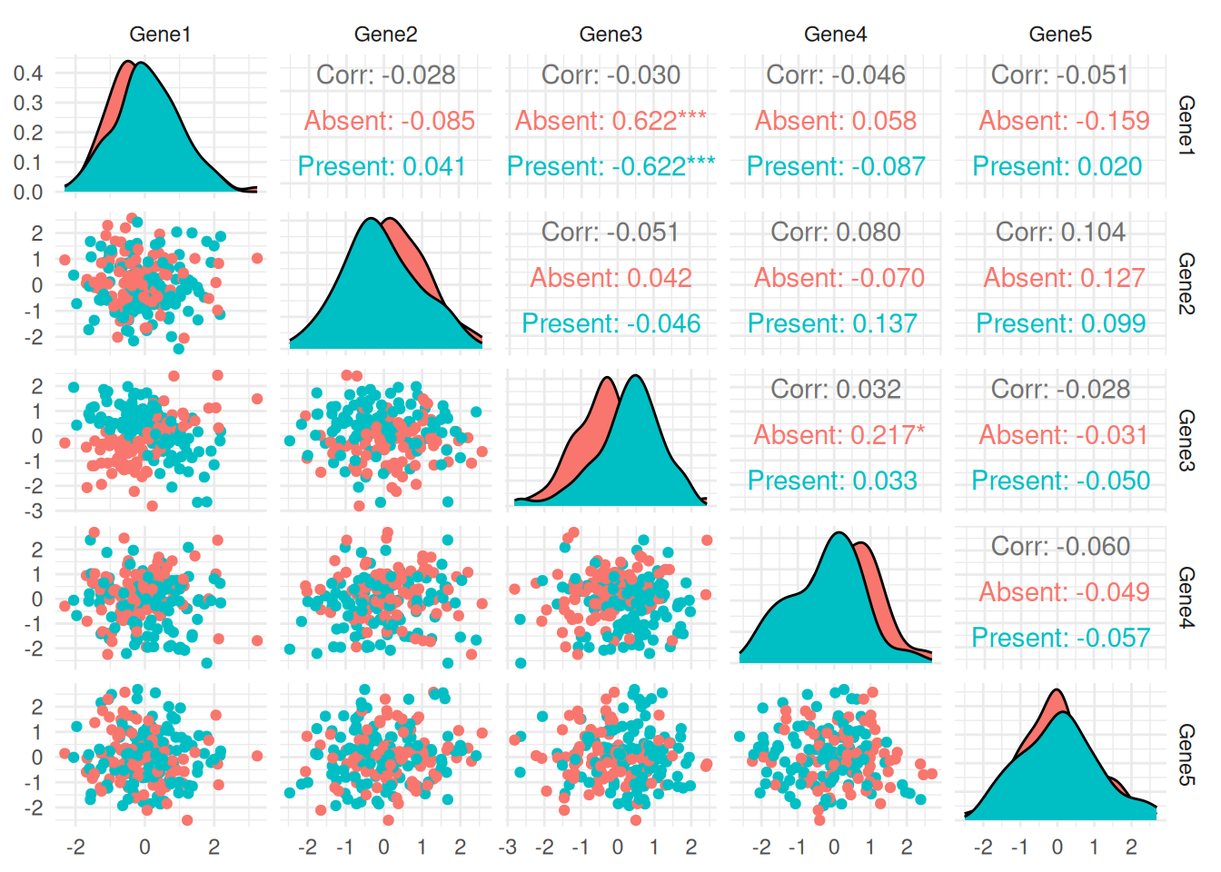
Modeling
We fit logistic regression and decision tree models to classify disease presence.
# Using logistic regression
logistic_model <- glm(disease_presence ~ ., data = bio_data, family = "binomial")

# Using rpart for classification
rpart_model <- rpart(disease_presence ~ ., data = bio_data, method = "class")
Evaluation
We evaluate and compare the accuracy of logistic regression and decision tree models.
# Predictions from models
logistic_pred <- predict(logistic_model, type = "response")
rpart_pred <- predict(rpart_model, type = "class", newdata = bio_data)

# Convert predictions to factors with levels
logistic_pred <- factor(ifelse(logistic_pred > 0.5, "Present", "Absent"), levels = c("Absent", "Present"))
rpart_pred <- factor(rpart_pred, levels = levels(disease_presence))

# Evaluate model performance (yardstick)
logistic_accuracy <- mean(logistic_pred == bio_data$disease_presence)
rpart_accuracy <- mean(rpart_pred == bio_data$disease_presence)

cat("Logistic Regression Accuracy:", logistic_accuracy, "\n")
Logistic Regression Accuracy: 0.74 cat("Decision Tree (rpart) Accuracy:", rpart_accuracy, "\n")Decision Tree (rpart) Accuracy: 0.905 # Plotting the decision tree
library(rpart.plot)
rpart.plot(rpart_model,type=5)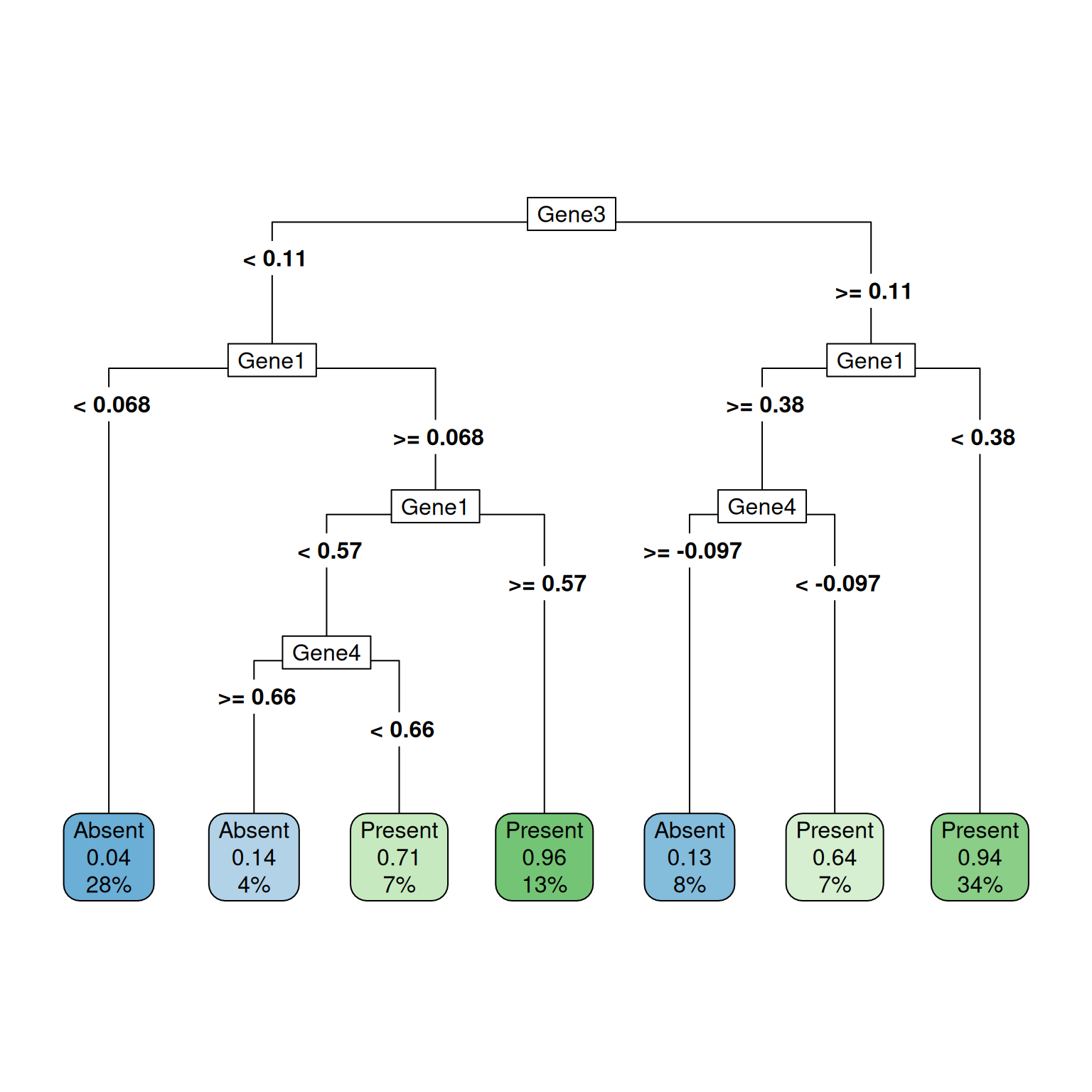
Summarize Logistic Regression Coefficients
# Summarizing logistic regression coefficients
summary(logistic_model)
Call:
glm(formula = disease_presence ~ ., family = "binomial", data = bio_data)

Coefficients:
            Estimate Std. Error z value Pr(>|z|)
(Intercept)  0.31891    0.16361   1.949 0.051277 .
Gene1        0.26941    0.17722   1.520 0.128464
Gene2       -0.24082    0.16551  -1.455 0.145672
Gene3        0.82736    0.18946   4.367 1.26e-05 ***
Gene4       -0.57850    0.17151  -3.373 0.000744 ***
Gene5        0.10475    0.16203   0.646 0.517959
Gene6        0.10762    0.16665   0.646 0.518408
Gene7        0.12048    0.17324   0.695 0.486788
Gene8        0.39470    0.18067   2.185 0.028912 *
Gene9       -0.12785    0.15425  -0.829 0.407174
Gene10      -0.07877    0.15804  -0.498 0.618189
---
Signif. codes:  0 '***' 0.001 '**' 0.01 '*' 0.05 '.' 0.1 ' ' 1

(Dispersion parameter for binomial family taken to be 1)

    Null deviance: 273.33  on 199  degrees of freedom
Residual deviance: 227.19  on 189  degrees of freedom
AIC: 249.19

Number of Fisher Scoring iterations: 4
# Decision boundary visualization
plot_decision_boundary <- function(model, data, feature1, feature2, model_type) {
# Create grid for visualization
grid <- expand.grid(
Feature1 = seq(min(data[[feature1]]) - 1, max(data[[feature1]]) + 1, length.out = 200),
Feature2 = seq(min(data[[feature2]]) - 1, max(data[[feature2]]) + 1, length.out = 200)
)
colnames(grid) <- c(feature1, feature2)
# Add the remaining variables as means
for (feature in setdiff(names(data), c(feature1, feature2, "disease_presence"))) {
grid[[feature]] <- mean(data[[feature]])
}
if (model_type == "logistic") {
grid$response <- predict(model, newdata = grid, type = "response")
grid$response <- factor(ifelse(grid$response > 0.5, "Present", "Absent"), levels = c("Absent", "Present"))
} else {
grid$response <- predict(model, newdata = grid, type = "class")
}
ggplot(data, aes(x = !!rlang::sym(feature1), y = !!rlang::sym(feature2))) +
geom_point(aes(fill = disease_presence), alpha = 1, shape = 21, col = "black", size = 3) +
geom_tile(
data = grid,
aes(x = !!rlang::sym(feature1), y = !!rlang::sym(feature2), fill = response),
alpha = 0.3,
inherit.aes = FALSE
) +
scale_fill_manual(values = c("Absent" = "turquoise", "Present" = "magenta")) +
scale_color_manual(values = c("Absent" = "turquoise", "Present" = "magenta")) +
theme_minimal() +
labs(title = paste("Decision Boundary for", model_type, "Model"), x = feature1, y = feature2)
}
# Decision boundary for Logistic Regression using Gene1 and Gene3
print(plot_decision_boundary(logistic_model, bio_data, "Gene1", "Gene3", "logistic"))Warning: No shared levels found between `names(values)` of the manual scale and the
data's colour values.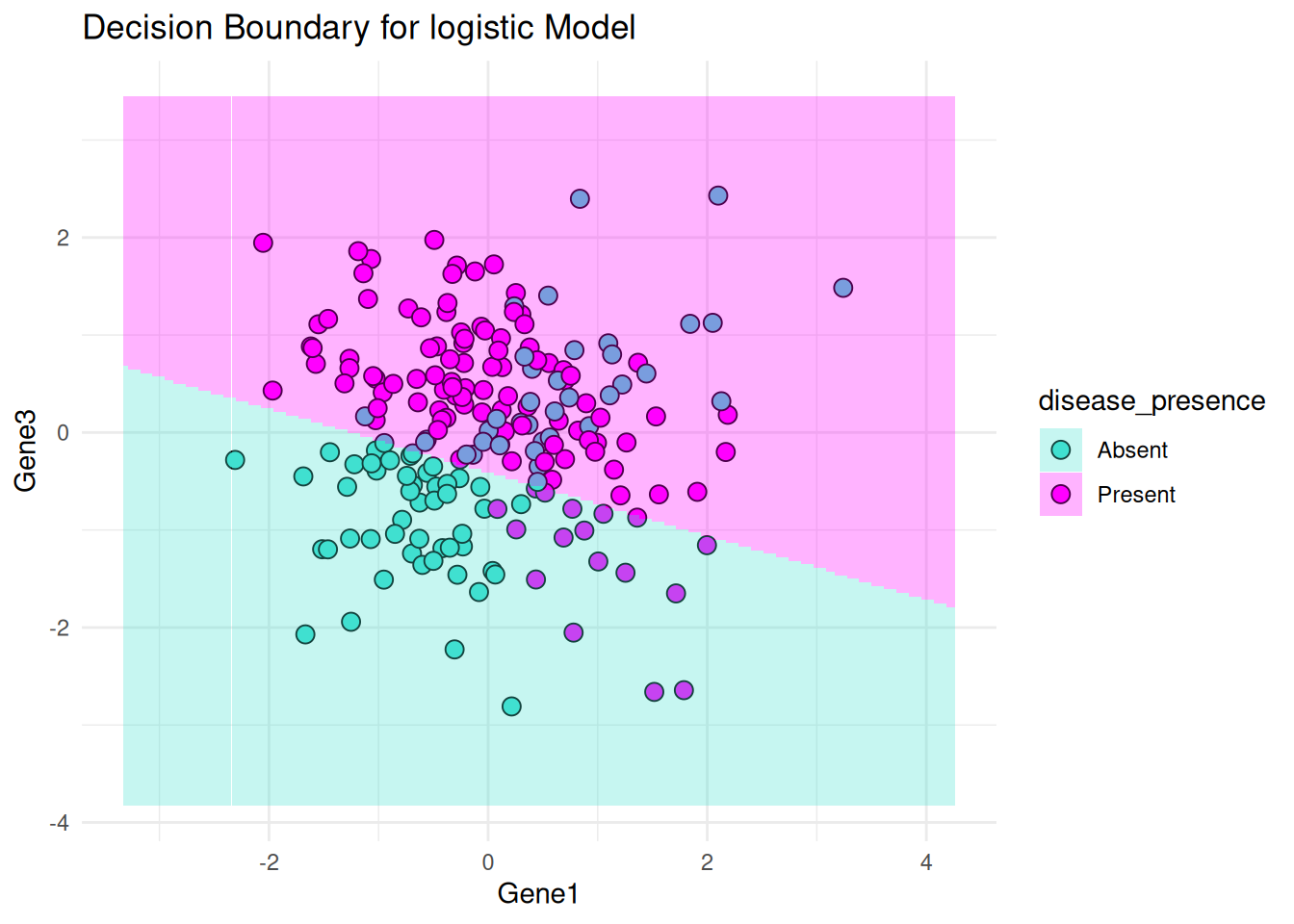
# Decision boundary for rpart using Gene1 and Gene3
print(plot_decision_boundary(rpart_model, bio_data, "Gene1", "Gene3", "rpart"))
Warning: No shared levels found between `names(values)` of the manual scale and the
data's colour values.