pg_sex <- palmerpenguins::penguins |>
  tidyr::drop_na(
    sex, bill_length_mm, bill_depth_mm,
    flipper_length_mm, body_mass_g, island, year
  ) |>
  mutate(
    sex = droplevels(sex),
    year = as.numeric(year)
  ) |>
select(-species)Palmer Penguins — SHAP walkthrough
Overview
Self-contained SHAP example on Palmer Penguins.
- Task: predict
sexfrom morphometrics + island/year (nospecies) - One model: random forest (
ranger) - SHAP outputs: beeswarm with individual points, mean absolute SHAP bar plot, and waterfall plots for individual penguins
Related: Module 06 SHAP section
Prepare data
pg_sex |>
  count(sex) |>
knitr::kable(col.names = c("Sex", "n"))| Sex | n |
|---|---|
| female | 165 |
| male | 168 |
Fit one explicit model (random forest)
rec_sex <- recipe(
  sex ~ bill_length_mm + bill_depth_mm + flipper_length_mm +
    body_mass_g + island + year,
  data = pg_sex
) |>
  step_zv(all_predictors()) |>
  step_dummy(all_nominal_predictors()) |>
  step_normalize(all_numeric_predictors())

rf_spec <- rand_forest(trees = 300, mtry = 3, min_n = 2) |>
  set_engine("ranger", probability = TRUE) |>
  set_mode("classification")

wf_sex <- workflow() |>
  add_recipe(rec_sex) |>
  add_model(rf_spec)

fit_sex <- fit(wf_sex, data = pg_sex)
Compute SHAP values explicitly
This section does the SHAP workflow in small steps:
- Extract trained preprocessing from the fitted workflow.
- Bake predictors so we get the numeric model matrix used by the forest.
- Choose a subset of rows to explain (
X_shap) and a background reference set (bg_X). - Define
pred_funto return P(male) from the fittedrangermodel. - Run
kernelshap()to estimate contributions, then wrap withshapviz(). - Identify one male and one female row for waterfall examples.
rec_est <- extract_recipe(fit_sex, estimated = TRUE)
X_model <- bake(rec_est, new_data = pg_sex, all_predictors())

set.seed(11)
X_shap <- dplyr::slice_sample(X_model, n = min(80, nrow(X_model)))
bg_X <- dplyr::slice_sample(X_model, n = min(35, nrow(X_model)))

rf_engine <- extract_fit_parsnip(fit_sex)$fit
pred_fun <- function(object, X_new) {
  as.numeric(predict(object, data = X_new)$predictions[, "male"])
}

ks <- kernelshap::kernelshap(rf_engine, X = X_shap, pred_fun = pred_fun, bg_X = bg_X)
  |
  |                                                                      |   0%
  |
  |=                                                                     |   1%
  |
  |==                                                                    |   2%
  |
  |===                                                                   |   4%
  |
  |====                                                                  |   5%
  |
  |====                                                                  |   6%
  |
  |=====                                                                 |   8%
  |
  |======                                                                |   9%
  |
  |=======                                                               |  10%
  |
  |========                                                              |  11%
  |
  |=========                                                             |  12%
  |
  |==========                                                            |  14%
  |
  |==========                                                            |  15%
  |
  |===========                                                           |  16%
  |
  |============                                                          |  18%
  |
  |=============                                                         |  19%
  |
  |==============                                                        |  20%
  |
  |===============                                                       |  21%
  |
  |================                                                      |  22%
  |
  |=================                                                     |  24%
  |
  |==================                                                    |  25%
  |
  |==================                                                    |  26%
  |
  |===================                                                   |  28%
  |
  |====================                                                  |  29%
  |
  |=====================                                                 |  30%
  |
  |======================                                                |  31%
  |
  |=======================                                               |  32%
  |
  |========================                                              |  34%
  |
  |========================                                              |  35%
  |
  |=========================                                             |  36%
  |
  |==========================                                            |  38%
  |
  |===========================                                           |  39%
  |
  |============================                                          |  40%
  |
  |=============================                                         |  41%
  |
  |==============================                                        |  42%
  |
  |===============================                                       |  44%
  |
  |================================                                      |  45%
  |
  |================================                                      |  46%
  |
  |=================================                                     |  48%
  |
  |==================================                                    |  49%
  |
  |===================================                                   |  50%
  |
  |====================================                                  |  51%
  |
  |=====================================                                 |  52%
  |
  |======================================                                |  54%
  |
  |======================================                                |  55%
  |
  |=======================================                               |  56%
  |
  |========================================                              |  58%
  |
  |=========================================                             |  59%
  |
  |==========================================                            |  60%
  |
  |===========================================                           |  61%
  |
  |============================================                          |  62%
  |
  |=============================================                         |  64%
  |
  |==============================================                        |  65%
  |
  |==============================================                        |  66%
  |
  |===============================================                       |  68%
  |
  |================================================                      |  69%
  |
  |=================================================                     |  70%
  |
  |==================================================                    |  71%
  |
  |===================================================                   |  72%
  |
  |====================================================                  |  74%
  |
  |====================================================                  |  75%
  |
  |=====================================================                 |  76%
  |
  |======================================================                |  78%
  |
  |=======================================================               |  79%
  |
  |========================================================              |  80%
  |
  |=========================================================             |  81%
  |
  |==========================================================            |  82%
  |
  |===========================================================           |  84%
  |
  |============================================================          |  85%
  |
  |============================================================          |  86%
  |
  |=============================================================         |  88%
  |
  |==============================================================        |  89%
  |
  |===============================================================       |  90%
  |
  |================================================================      |  91%
  |
  |=================================================================     |  92%
  |
  |==================================================================    |  94%
  |
  |==================================================================    |  95%
  |
  |===================================================================   |  96%
  |
  |====================================================================  |  98%
  |
  |===================================================================== |  99%
  |
  |======================================================================| 100%
shp <- shapviz::shapviz(ks, X_pred = X_shap)
sex_sample <- pg_sex$sex[as.integer(rownames(X_shap))]
male_row <- which(sex_sample == "male")[1]
female_row <- which(sex_sample == "female")[1]What positive/negative SHAP means
- We explain P(male), so each SHAP value is a push on that probability scale.
- Positive SHAP value: this feature pushes the prediction toward male (higher P(male)).
- Negative SHAP value: this feature pushes the prediction away from male (toward female).
- In a waterfall plot, baseline + all SHAP contributions = final model output for that row.
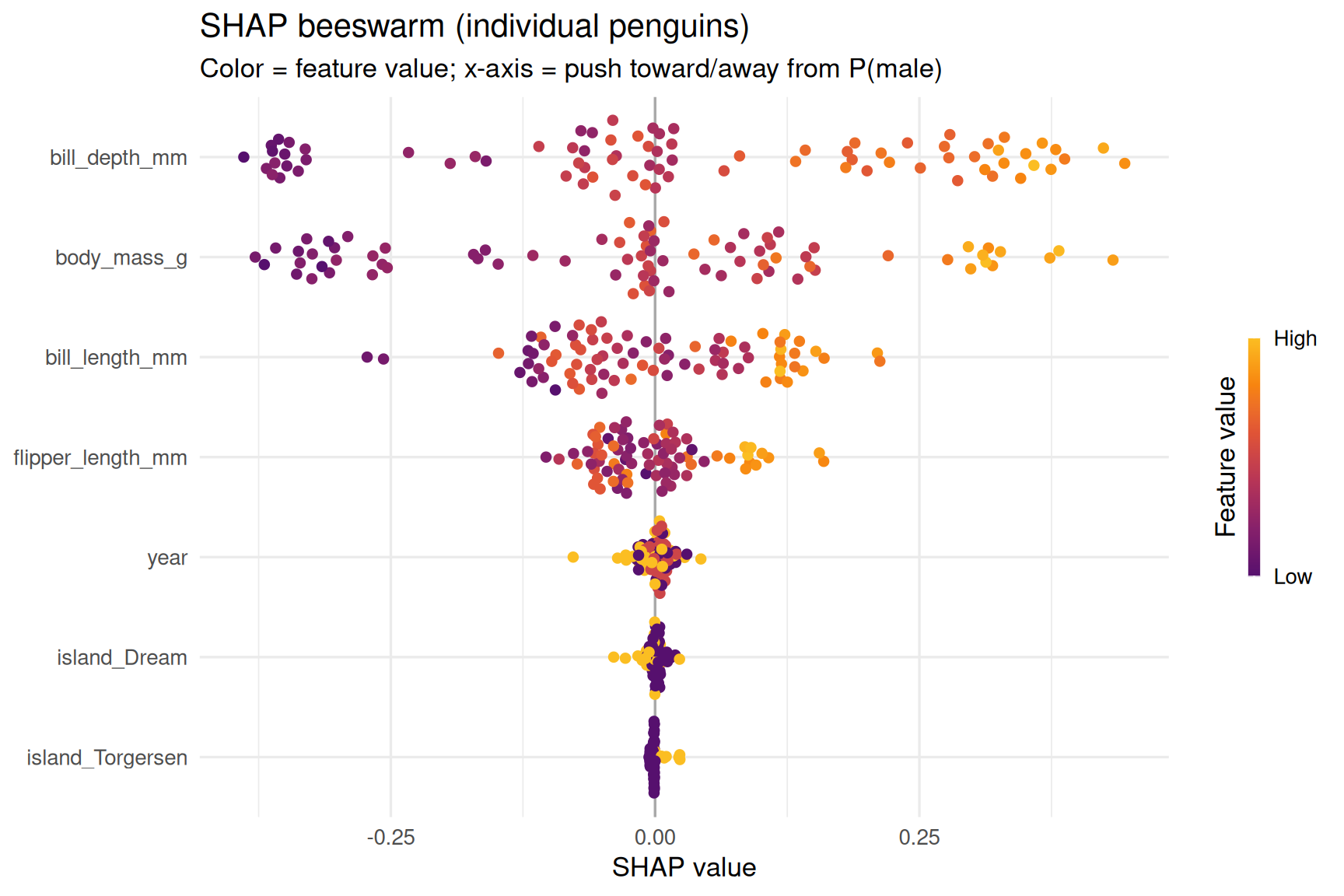
SHAP beeswarm (individual points)
Each dot is one penguin; horizontal position is SHAP contribution.
shapviz::sv_importance(
  shp,
  kind = "beeswarm",
  max_display = 12
) +
  theme_minimal(base_size = 13) +
  labs(
    title = "SHAP beeswarm (individual penguins)",
    subtitle = "Color = feature value; x-axis = push toward/away from P(male)"
  )
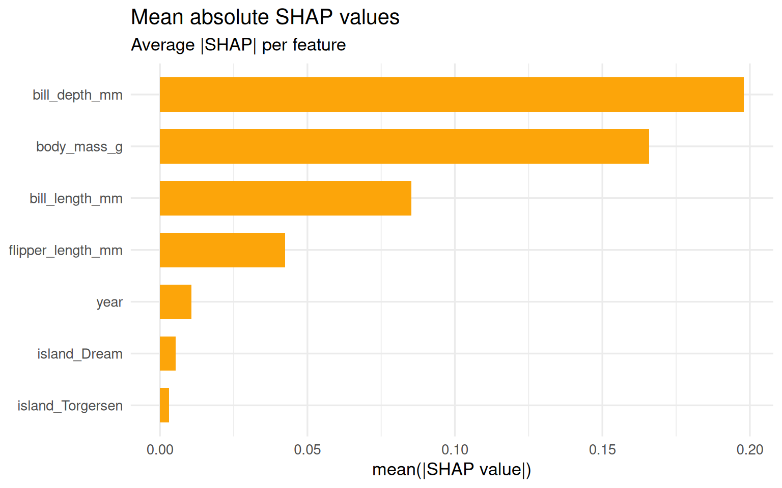
Mean absolute SHAP values (global importance)
This aggregates absolute contributions across rows.
shapviz::sv_importance(
  shp,
  kind = "bar",
  max_display = 12
) +
  theme_minimal(base_size = 13) +
  labs(
    title = "Mean absolute SHAP values",
    subtitle = "Average |SHAP| per feature"
  )
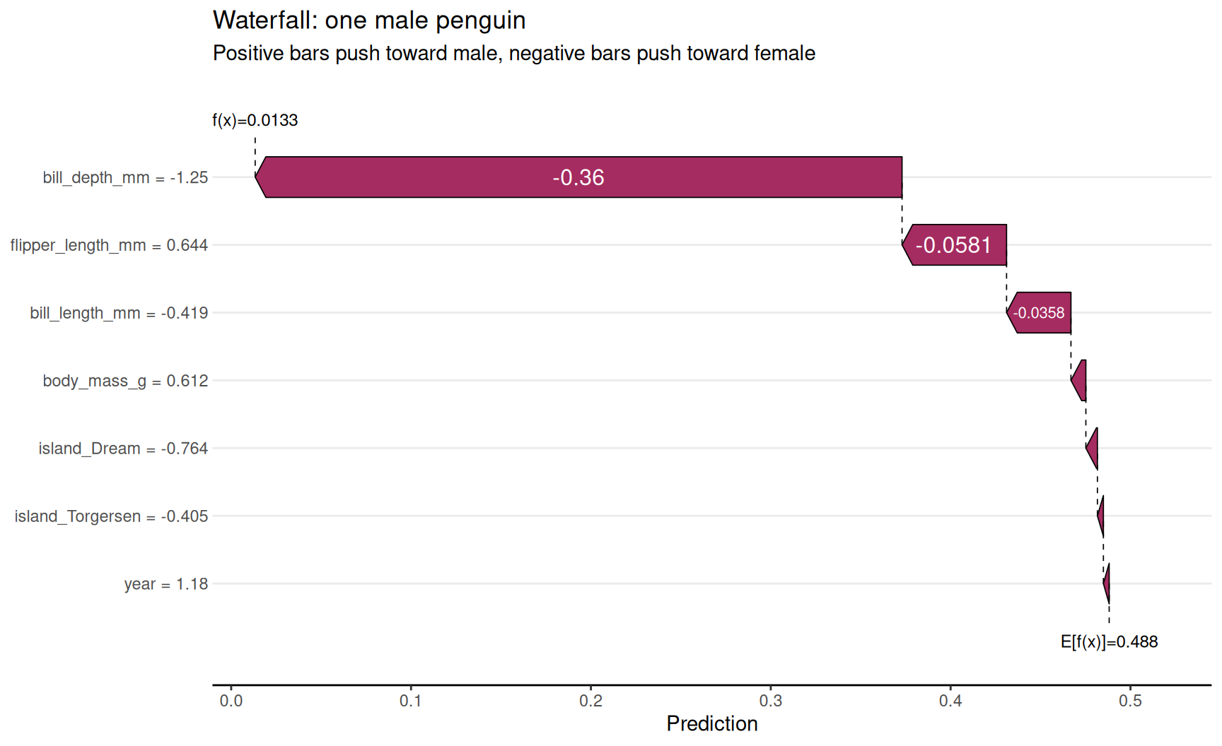
Waterfall plot for individual penguins
Example 1 — one male penguin
shapviz::sv_waterfall(
  shp,
  row_id = male_row
) +
  labs(
    title = "Waterfall: one male penguin",
    subtitle = "Positive bars push toward male, negative bars push toward female"
  )
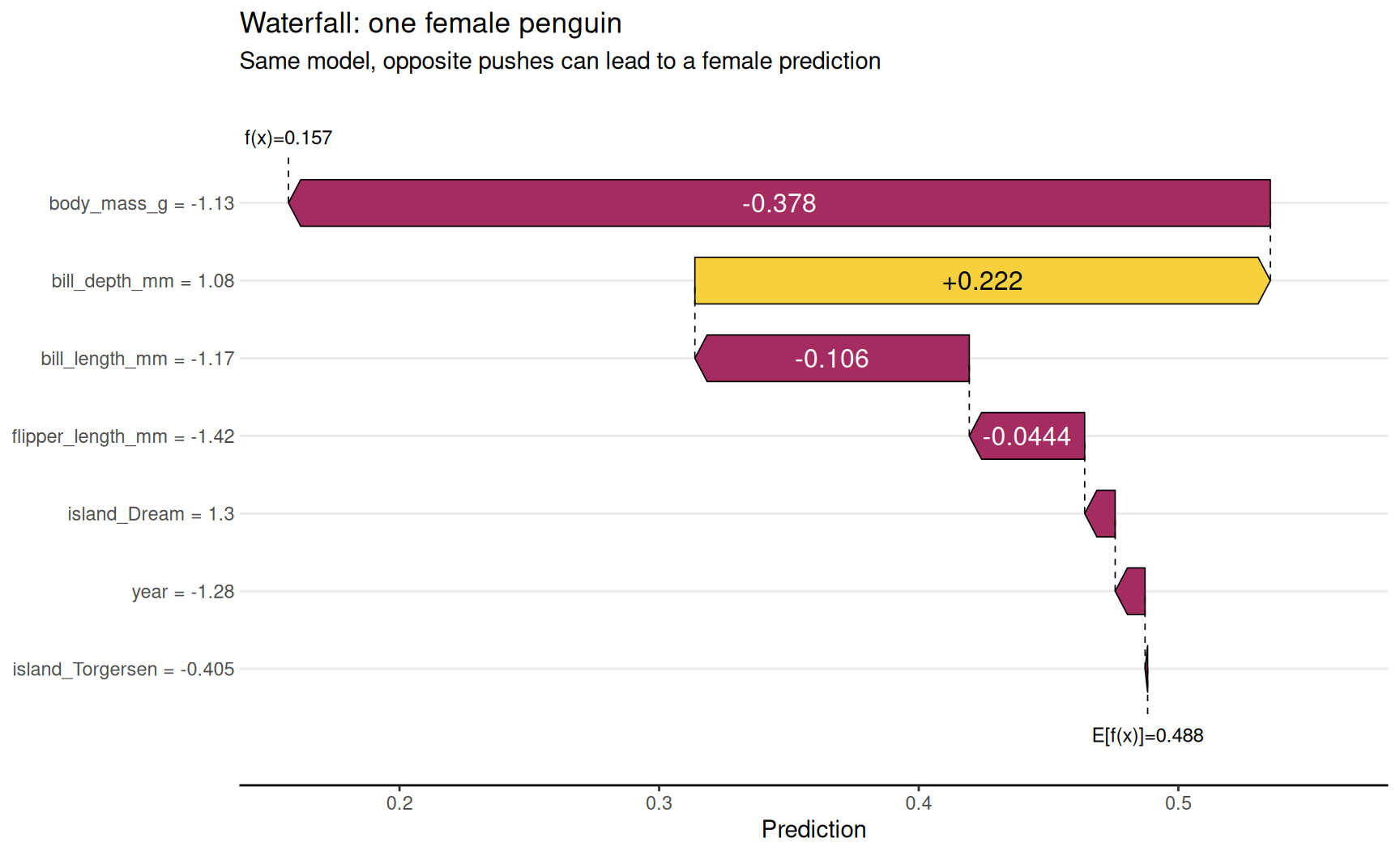
Example 2 — one female penguin
shapviz::sv_waterfall(
  shp,
  row_id = female_row
) +
  labs(
    title = "Waterfall: one female penguin",
    subtitle = "Same model, opposite pushes can lead to a female prediction"
  )
Quick interpretation checklist
- Beeswarm = distribution of local effects across many rows
- Mean |SHAP| bar = global ranking of influential features
- Waterfall = local explanation for one row only
- SHAP explains this fitted model; it does not prove causality