---
title: "Palmer Penguins — predicting sex (binary)"
author: "Aparna Pandey and Stephan Peischl"
format:
html:
toc: true
code-tools: true
engine: knitr
---
```{r setup, include=FALSE}
knitr::opts_chunk$set(echo = TRUE, message = FALSE, warning = FALSE)
library(palmerpenguins)
library(dplyr)
library(ggplot2)
library(GGally)
library(rpart)
library(rpart.plot)
library(tidymodels)
library(tidyr)
library(rlang)
theme_set(theme_classic())
```
# Overview
This notebook predicts **`sex`** (female vs male) from **morphometrics and island / year only**. We **deliberately omit `species`** as a predictor so the task is not trivially solved by species–sex composition differences alone (in exercises you can add `species` and compare accuracy — then discuss **leakage** and what you are willing to claim scientifically).
**Models:** `glm` and `rpart`. **Train/test split and confusion tables:** `tidymodels` (`initial_split`, `yardstick::conf_mat`). For a full Adelie-vs-Gentoo pipeline, see [Module 04](../modules/module-04-pipeline.qmd#train-test-last-fit).
See **[Palmer Penguins data card](../data/cards/palmer-penguins.qmd)** and the related notebooks (mass, species, multiclass). For **SHAP** on this task (without `species`), see [Module 06](../modules/module-06-evaluation-and-interpretability.qmd#shap-shapley-values-on-penguins-sex) and [Day 4 slides](../slides/day-04-thursday.html).
## Prepare data (complete cases on `sex`)
```{r}
data("penguins", package = "palmerpenguins")
pg <- penguins |>
  tidyr::drop_na(sex, bill_length_mm, bill_depth_mm, flipper_length_mm, body_mass_g, island, year) |>
  mutate(
    sex = droplevels(sex),
    year = as.numeric(year)
  ) |>
  dplyr::select(-species)

table(pg$sex)
nrow(pg)
```
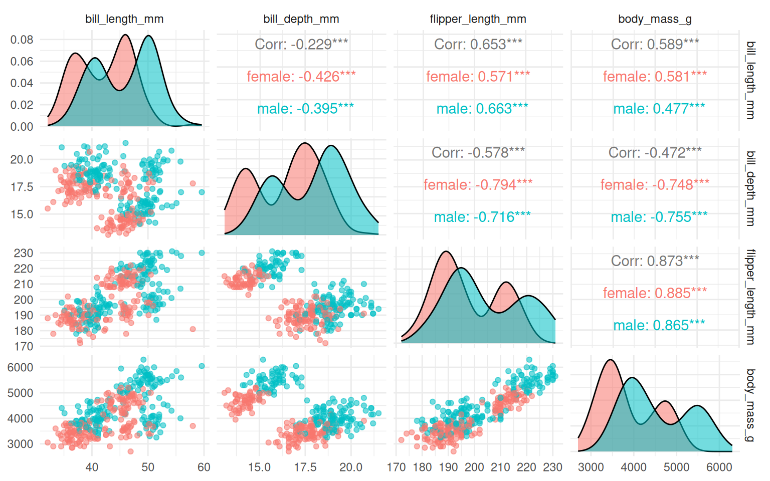
## Pair plot (measurements coloured by sex)
```{r fig.width=8, fig.height=5}
GGally::ggpairs(
  pg,
  columns = c("bill_length_mm", "bill_depth_mm", "flipper_length_mm", "body_mass_g"),
  aes(color = sex, alpha = 0.35)
) +
  theme_minimal()
```
## Train / test split (stratified on `sex`)
```{r}
set.seed(11)
split <- initial_split(pg, prop = 0.75, strata = sex)
train <- training(split)
test <- testing(split)
```
## Logistic regression (no `species` in formula)
```{r}
log_fit <- glm(
  sex ~ bill_length_mm + bill_depth_mm + flipper_length_mm + body_mass_g + island + year,
  data = train,
  family = binomial()
)
summary(log_fit)
```
```{r}
p_test <- predict(log_fit, newdata = test, type = "response")
pred_sex <- factor(ifelse(p_test > 0.5, levels(train$sex)[2], levels(train$sex)[1]), levels = levels(train$sex))
tibble(truth = test$sex, .pred_class = pred_sex) |>
  conf_mat(truth = truth, estimate = .pred_class)
```
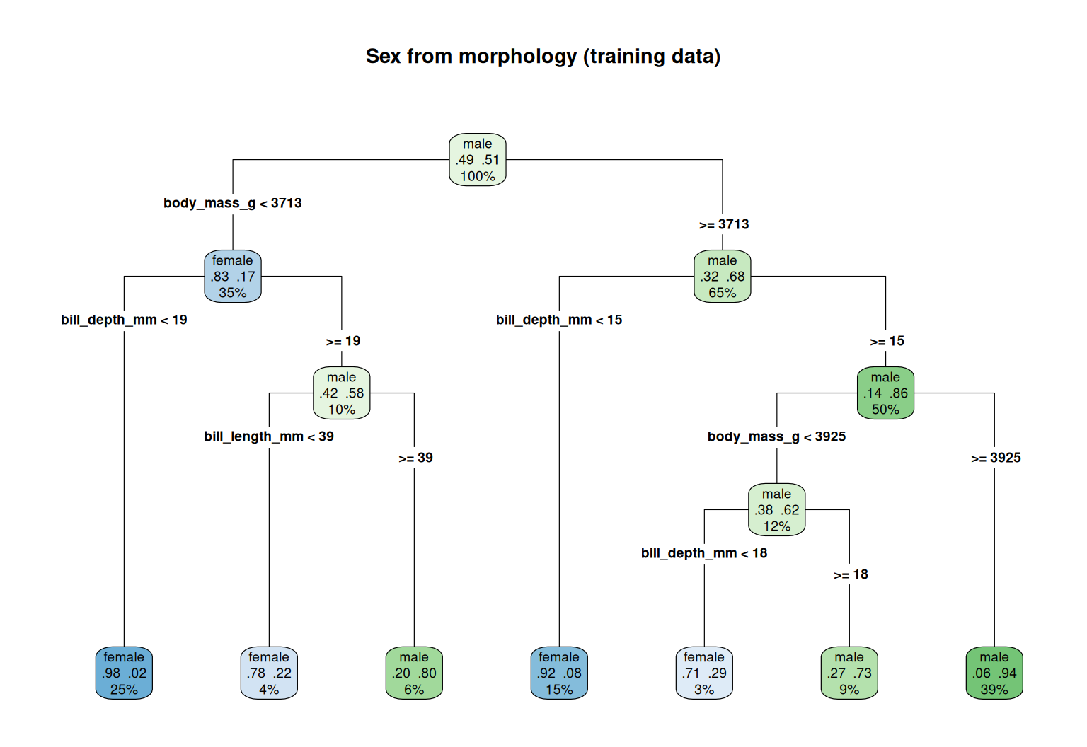
## Classification tree
```{r fig.width=8, fig.height=5.5}
tree_fit <- rpart(
  sex ~ bill_length_mm + bill_depth_mm + flipper_length_mm + body_mass_g + island + year,
  data = train,
  method = "class"
)
rpart.plot(tree_fit, type = 4, extra = 104, main = "Sex from morphology (training data)")
```
```{r}
pred_t <- predict(tree_fit, test, type = "class") |> factor(levels = levels(test$sex))
tibble(truth = test$sex, .pred_class = pred_t) |>
  conf_mat(truth = truth, estimate = .pred_class)
```
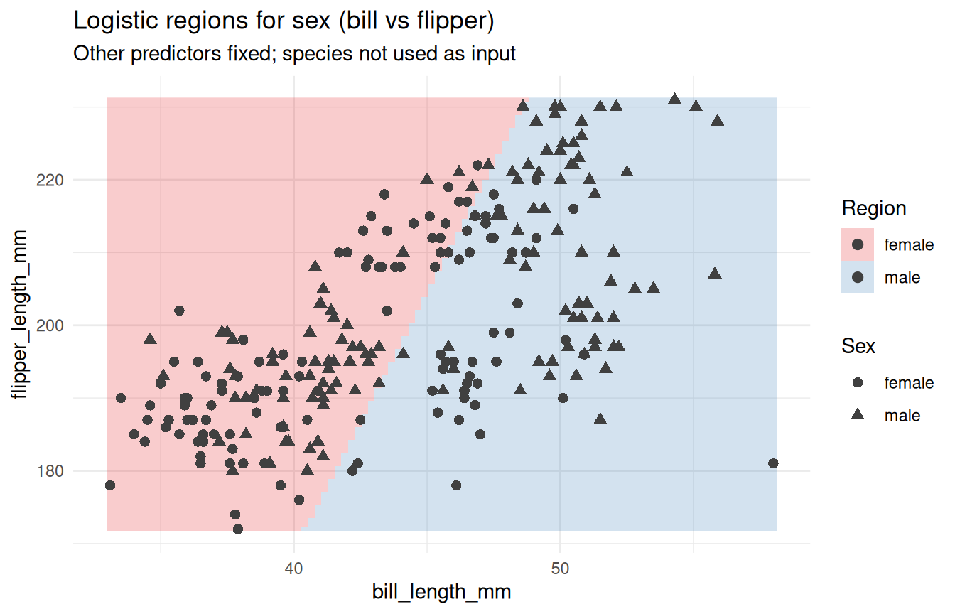
## 2D view (bill length vs flipper; other predictors at training medians / modes)
```{r fig.width=7, fig.height=4.5}
plot_boundary <- function(model, data, f1, f2) {
  r1 <- range(data[[f1]])
  r2 <- range(data[[f2]])
  grid <- expand.grid(
    seq(r1[1], r1[2], length.out = 100),
    seq(r2[1], r2[2], length.out = 100)
  )
  names(grid) <- c(f1, f2)
  for (nm in setdiff(names(data), c(f1, f2, "sex"))) {
    v <- data[[nm]]
    grid[[nm]] <- if (is.numeric(v)) stats::median(v, na.rm = TRUE) else {
      tab <- table(v)
      names(tab)[which.max(tab)]
    }
  }
  grid$p_male <- predict(model, newdata = grid, type = "response")
  lv <- levels(data$sex)
  grid$cls <- factor(ifelse(grid$p_male > 0.5, lv[2], lv[1]), levels = lv)
  ggplot(data, aes(!!sym(f1), !!sym(f2))) +
    geom_raster(data = grid, aes(!!sym(f1), !!sym(f2), fill = cls), alpha = 0.22, inherit.aes = FALSE) +
    geom_point(aes(shape = sex, fill = sex), size = 2.2, color = "gray25") +
    scale_fill_brewer(palette = "Set1") +
    theme_minimal() +
    labs(
      title = "Logistic regions for sex (bill vs flipper)",
      subtitle = "Other predictors fixed; species not used as input",
      fill = "Region", shape = "Sex"
    )
}
print(plot_boundary(log_fit, train, "bill_length_mm", "flipper_length_mm"))
```
## Takeaways
- **Missing `sex`** shrinks usable *n* — discuss NA reporting and whether imputation is defensible.
- Omitting **`species`** makes errors more interesting; adding it back is a one-line **ablation** for discussion.
- Compare difficulty here to **Adelie vs Gentoo** in `penguins-classification.Rmd`.