# Generate the dataset
# Set seed for reproducibility
set.seed(420)

# Number of samples
n <- 150

# Number of genes (variables)
p <- 10

# Generate gene names
gene_names <- c("GeneA", "GeneB", "GeneC", "GeneD", "GeneE", "GeneF", "GeneG", "GeneH", "GeneI", "GeneJ")

# Generate gene expression levels
gene_data <- matrix(rnorm(n * p), nrow = n)
colnames(gene_data) <- gene_names

# Trait influenced by GeneA and GeneB
trait <- -0.5 * gene_data[, "GeneA"] + 0.8 * gene_data[, "GeneB"] + rnorm(n, sd = 0.3)

# Noise genes correlated with trait but not causally related
gene_data[, "GeneC"] <- gene_data[, "GeneA"] + rnorm(n, sd = 0.2)
gene_data[, "GeneD"] <- -0.3 * gene_data[, "GeneB"] + rnorm(n, sd = 0.2)

# Add more irrelevant noise genes
for (i in 5:p) {
  gene_data[, gene_names[i]] <- rnorm(n)
}

# Introduce correlations among genes
gene_data[, "GeneF"] <- gene_data[, "GeneE"] + rnorm(n, sd = 0.2)
gene_data[, "GeneH"] <- -0.5 * gene_data[, "GeneG"] + rnorm(n, sd = 0.2)

# Add a strong correlation between an irrelevant gene and a relevant gene
gene_data[, "GeneJ"] <- 0.7 * gene_data[, "GeneA"] + rnorm(n, sd = 0.2)

# Combine gene data and trait into a single data frame
data <- as.data.frame(cbind(gene_data, trait))Linear Regression, Model Selection and LASSO example
Automatic feature seleciton
The goal of this notebook is to illustrate Lasso and Model selection based on AIC.
We use a synthetic dataset for illustrative purposes. This has the advantage that we know exactly what’s going on.
Concept companion (short read on the site): Module 02 — Regularization frames ridge, lasso, and AIC in the same vocabulary as Monday’s slides — run this notebook when you want the long runnable lab.
In this simulated dataset, GeneA and GeneB are genes that directly influence a specific biological trait, while GeneC and GeneD are noise genes that are correlated with the trait but do not contribute causally. GeneJ is in strongly correlated to GeneA but not causally linked to the trait. Other genes act as irrelevant noise variables or have correlations among themselves.
- The training and testing data splits are created.
- The data is preprocessed by standardizing the features.
- LASSO regression is applied to the training data using cv.glmnet to determine the best lambda value.
- The model is then trained with the best lambda value.
- Prediction is made on the test data, and evaluation metrics such as MSE, RMSE, and R-squared are calculated.
- Backward and forward model selection using AIC are performed to find the best model.
- Predictions are made with the selected models, and evaluation metrics are calculated for both models.
Generate and visualize the dataset
Visualize our data:
# Create a scatterplot matrix using ggpairs
ggpairs(data,
        upper = list(continuous = wrap("cor", size = 2.5)),
        aes(alpha = 0.1)) +
  theme(axis.text.x = element_text(angle = 45, hjust = 1)) +
  theme(axis.text.y = element_text(angle = 0, hjust = 1))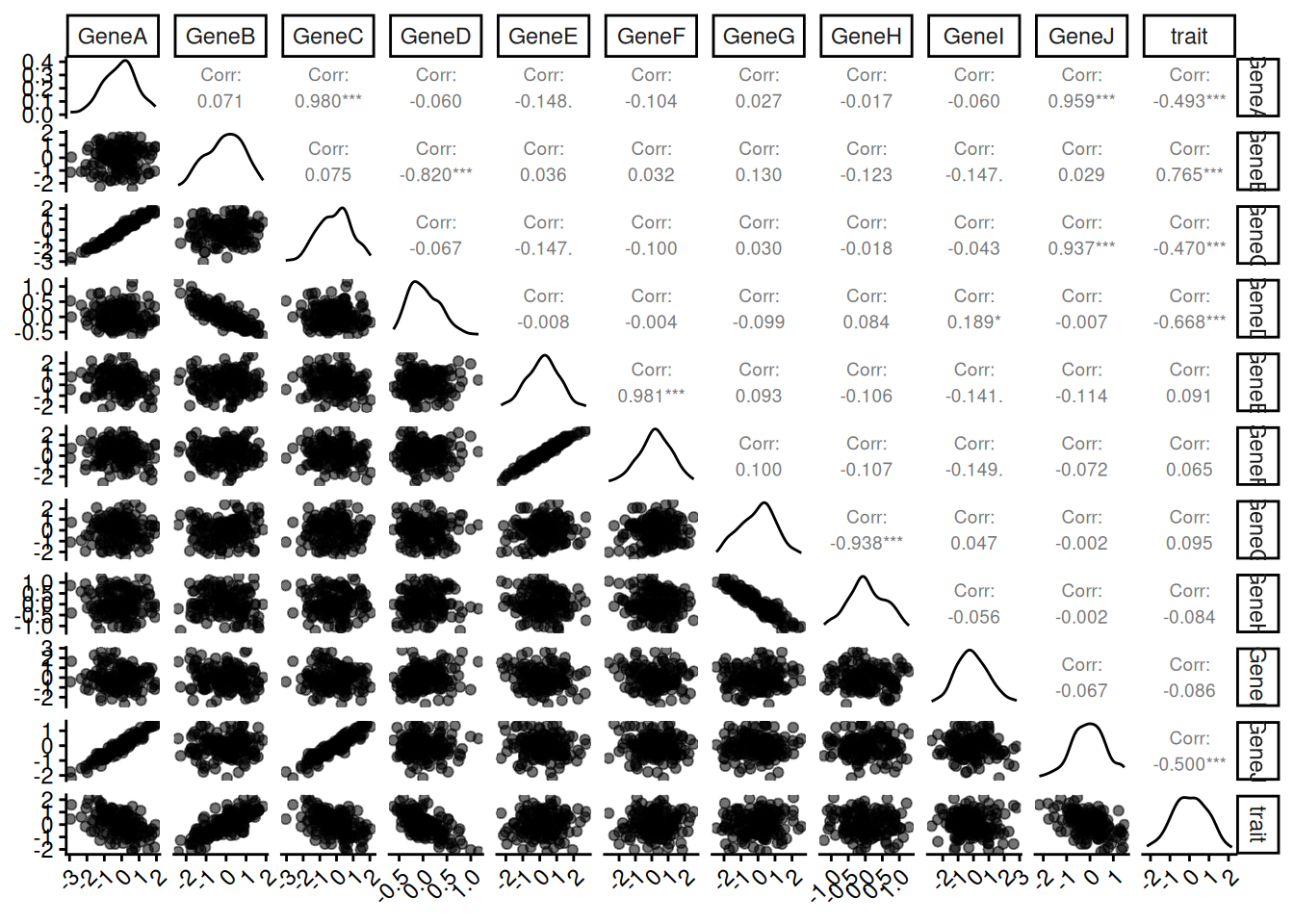
# Calculate the correlation matrix
correlation_matrix <- cor(data)

# Convert the correlation matrix to a long format for plotting
cor_data <- as.data.frame(as.table(correlation_matrix)) %>%
  rename(variable1 = Var1, variable2 = Var2, correlation = Freq)

# Create the plot using ggplot
ggplot(cor_data, aes(variable1, variable2, fill = correlation)) +
  geom_tile(color = "white") +
  scale_fill_gradient2(low = "dodgerblue", high = "firebrick4", mid = "white",midpoint = 0, limit = c(-1,1), space = "Lab",
                       name="Correlation") +
  theme_minimal() +
  theme(axis.text.x = element_text(angle = 45, hjust = 1)) +
  coord_fixed()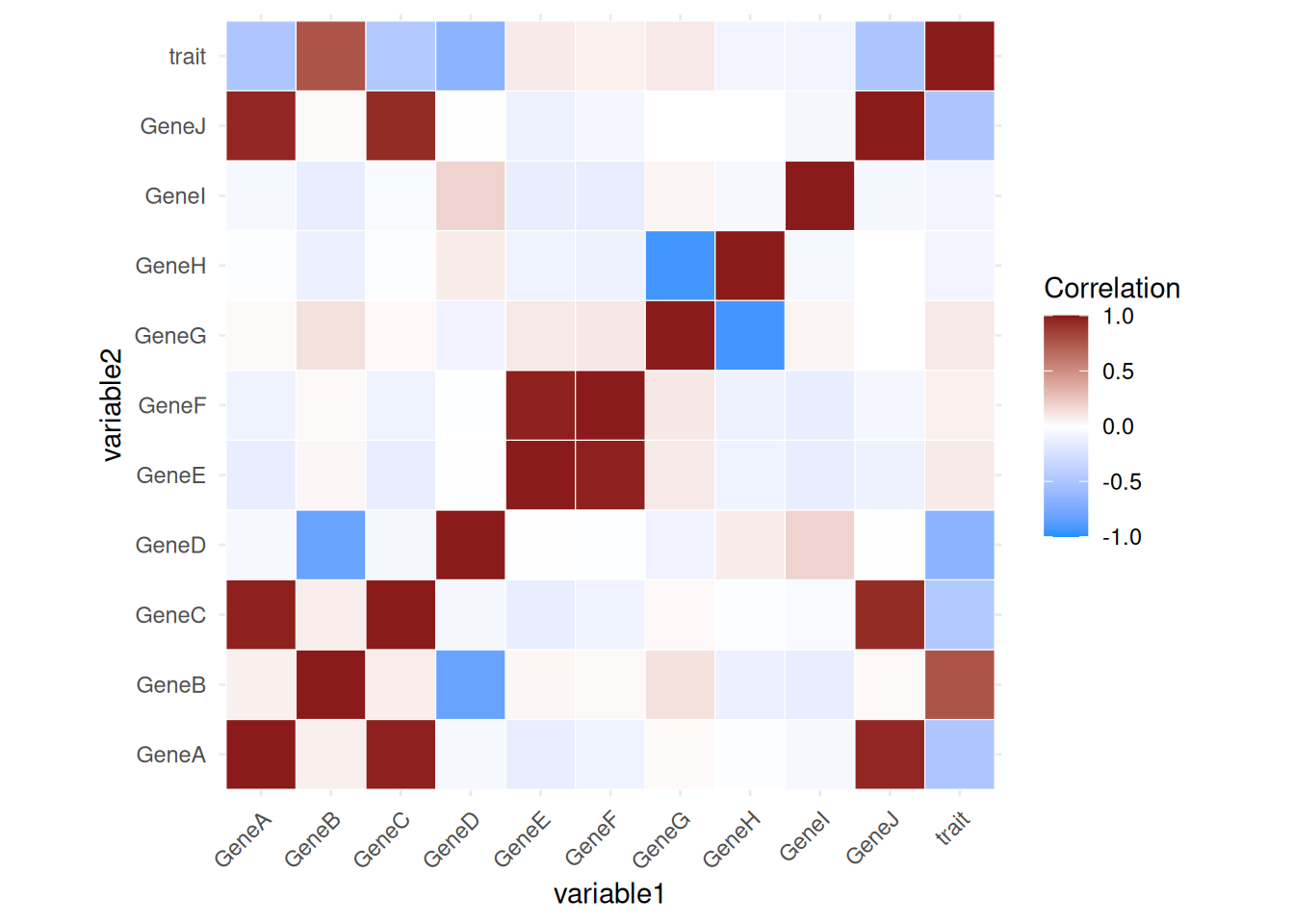
Fit a LASSO model
We now split the data into test and training, and then fit a Lasso model and test it’s precision on a test dataset.
set.seed(123)
split <- initial_split(data, prop = 0.8)
train <- training(split)
test <- testing(split)

rec_scale <- recipe(trait ~ ., data = train) |>
  step_normalize(all_numeric_predictors())
prep_fit <- prep(rec_scale, train)
train_scaled <- bake(prep_fit, train)
test_scaled <- bake(prep_fit, test)

X_train_scaled <- as.matrix(dplyr::select(train_scaled, -trait))
y_train <- train_scaled$trait
X_test_scaled <- as.matrix(dplyr::select(test_scaled, -trait))
y_test <- test_scaled$trait

# Apply LASSO regression
# alpha=1 for LASSO in glmnet

lasso_model <- cv.glmnet(X_train_scaled, y_train, alpha = 1,lambda =  10^seq(-3, -0.1, length = 20))  #


# Plot the cross-validation results to choose the best lambda
plot(lasso_model,log="y",ylim = c(0.03,0.2))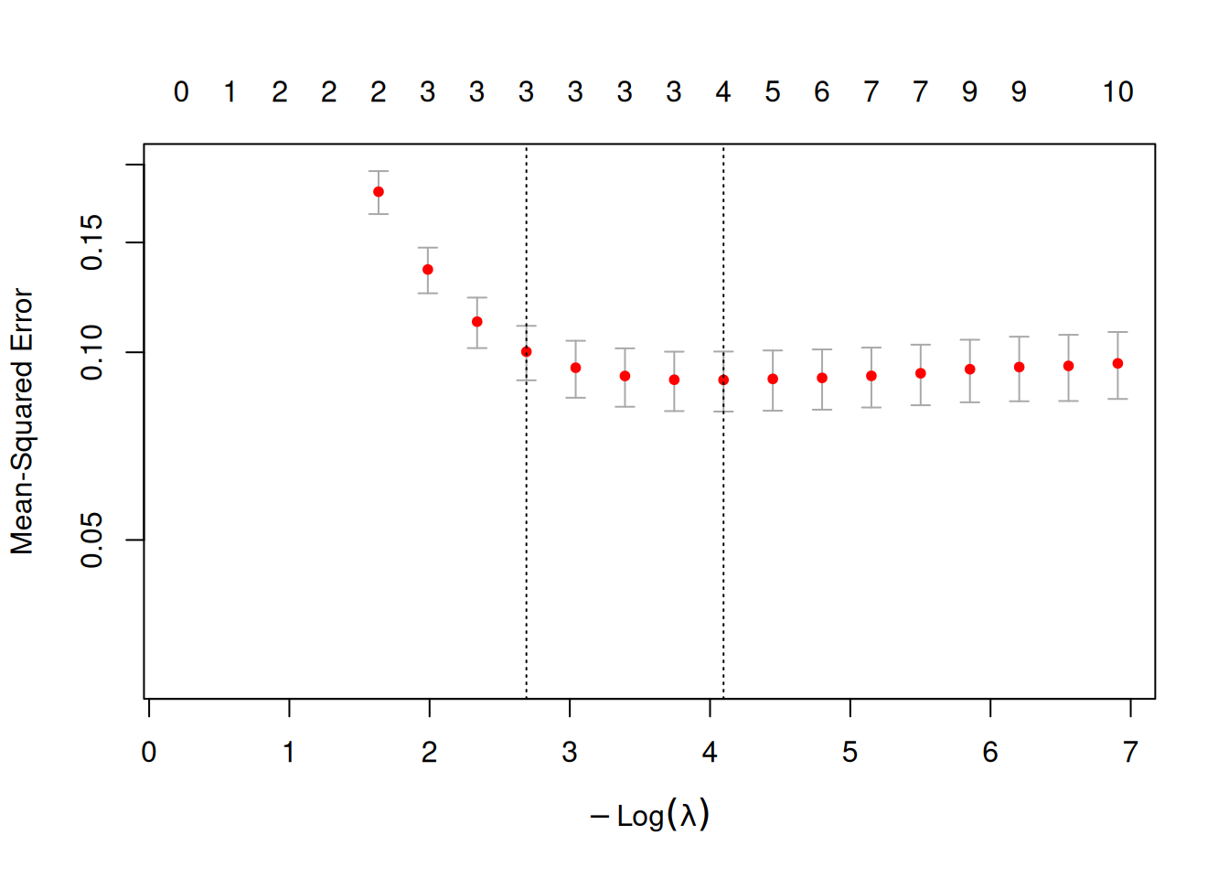
best_lambda <- lasso_model$lambda.1se


# Fit the model with the best lambda
lasso_best <- glmnet(X_train_scaled, y_train, alpha = 1, lambda = best_lambda)

# Print the coefficients
coef(lasso_best)
11 x 1 sparse Matrix of class "dgCMatrix"
s0
(Intercept) 0.04323495
GeneA -0.40339647
GeneB 0.62317164
GeneC .
GeneD -0.06971150
GeneE .
GeneF .
GeneG .
GeneH .
GeneI .
GeneJ . # Predict on the test data
y_pred <- predict(lasso_best, newx = X_test_scaled)
# Calculate evaluation metrics
mse_lasso <- mean((y_test - y_pred)^2)
rmse_lasso <- sqrt(mse_lasso)
r2_lasso <- cor(y_test, y_pred)^2Forward and Backward model selection
Now we do the same, but we use forward and backward selection using AIC.
library(MASS)
Attaching package: 'MASS'The following object is masked from 'package:dplyr':
selectX_train = as.data.frame(X_train_scaled)
X_test = as.data.frame(X_test_scaled)
X_train = mutate(X_train,trait = y_train)
X_test = mutate(X_test,trait = y_test)
# Backward selection using AIC
full_model <- lm(trait ~ ., data = X_train)
backward_model <- stepAIC(full_model, direction = "backward", trace = FALSE)
summary(backward_model)
Call:
lm(formula = trait ~ GeneA + GeneB + GeneD, data = X_train)

Residuals:
     Min       1Q   Median       3Q      Max
-0.70274 -0.22462 -0.00915  0.19965  0.83177

Coefficients:
            Estimate Std. Error t value Pr(>|t|)
(Intercept)  0.04323    0.02672   1.618   0.1084
GeneA       -0.47907    0.02696 -17.769   <2e-16 ***
GeneB        0.66480    0.04743  14.015   <2e-16 ***
GeneD       -0.11032    0.04742  -2.327   0.0217 *
---
Signif. codes:  0 '***' 0.001 '**' 0.01 '*' 0.05 '.' 0.1 ' ' 1

Residual standard error: 0.2927 on 116 degrees of freedom
Multiple R-squared:  0.898, Adjusted R-squared:  0.8954
F-statistic: 340.4 on 3 and 116 DF,  p-value: < 2.2e-16
# Forward selection using AIC
# Start with an empty model
start_model <- lm(trait ~ 1, data = X_train)
forward_model <- stepAIC(start_model, direction = "forward", scope = list(lower = start_model, upper = full_model), trace = FALSE)
summary(forward_model)
Call:
lm(formula = trait ~ GeneB + GeneA + GeneD, data = X_train)

Residuals:
     Min       1Q   Median       3Q      Max
-0.70274 -0.22462 -0.00915  0.19965  0.83177

Coefficients:
            Estimate Std. Error t value Pr(>|t|)
(Intercept)  0.04323    0.02672   1.618   0.1084
GeneB        0.66480    0.04743  14.015   <2e-16 ***
GeneA       -0.47907    0.02696 -17.769   <2e-16 ***
GeneD       -0.11032    0.04742  -2.327   0.0217 *
---
Signif. codes:  0 '***' 0.001 '**' 0.01 '*' 0.05 '.' 0.1 ' ' 1

Residual standard error: 0.2927 on 116 degrees of freedom
Multiple R-squared:  0.898, Adjusted R-squared:  0.8954
F-statistic: 340.4 on 3 and 116 DF,  p-value: < 2.2e-16