---
title: "Penguins: why logistic `glm` may not converge"
author: "Aparna Pandey and Stephan Peischl"
format:
html:
toc: true
code-tools: true
engine: knitr
---
```{r setup, include=FALSE}
knitr::opts_chunk$set(echo = TRUE, message = FALSE, warning = FALSE)
suppressPackageStartupMessages({
library(tidymodels)
library(palmerpenguins)
library(dplyr)
library(ggplot2)
library(glmnet)
})
theme_set(theme_minimal(base_size = 13))
```
## Goal
Short explanation of a common warning in logistic regression:
- `glm.fit: algorithm did not converge`
- or probabilities numerically at `0` / `1`
This usually appears when the model can (almost) **separate** classes, especially with many predictors and limited sample size.
## 1) A normal logistic model (usually converges)
```{r data}
peng <- penguins |>
  filter(species %in% c("Adelie", "Gentoo")) |>
  mutate(
    y = factor(species, levels = c("Adelie", "Gentoo")),
    year = as.numeric(year)
  ) |>
  select(y, bill_length_mm, bill_depth_mm, flipper_length_mm, body_mass_g, island, sex, year) |>
  drop_na()

nrow(peng)
```
```{r glm-ok}
m_ok <- glm(
  y ~ bill_length_mm + bill_depth_mm + flipper_length_mm + body_mass_g + island + sex + year,
  data = peng,
  family = binomial
)

m_ok$converged
summary(m_ok)$coefficients |> head()
```
## 1.5) 1D intuition: steeper and steeper logistic curves
In 1D, logistic regression fits
\[
\Pr(y=1 \mid x)=\text{logit}^{-1}(\beta_0 + \beta_1 x).
\]
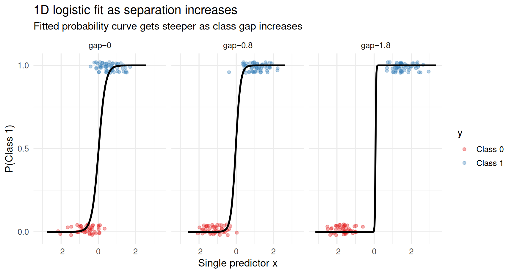
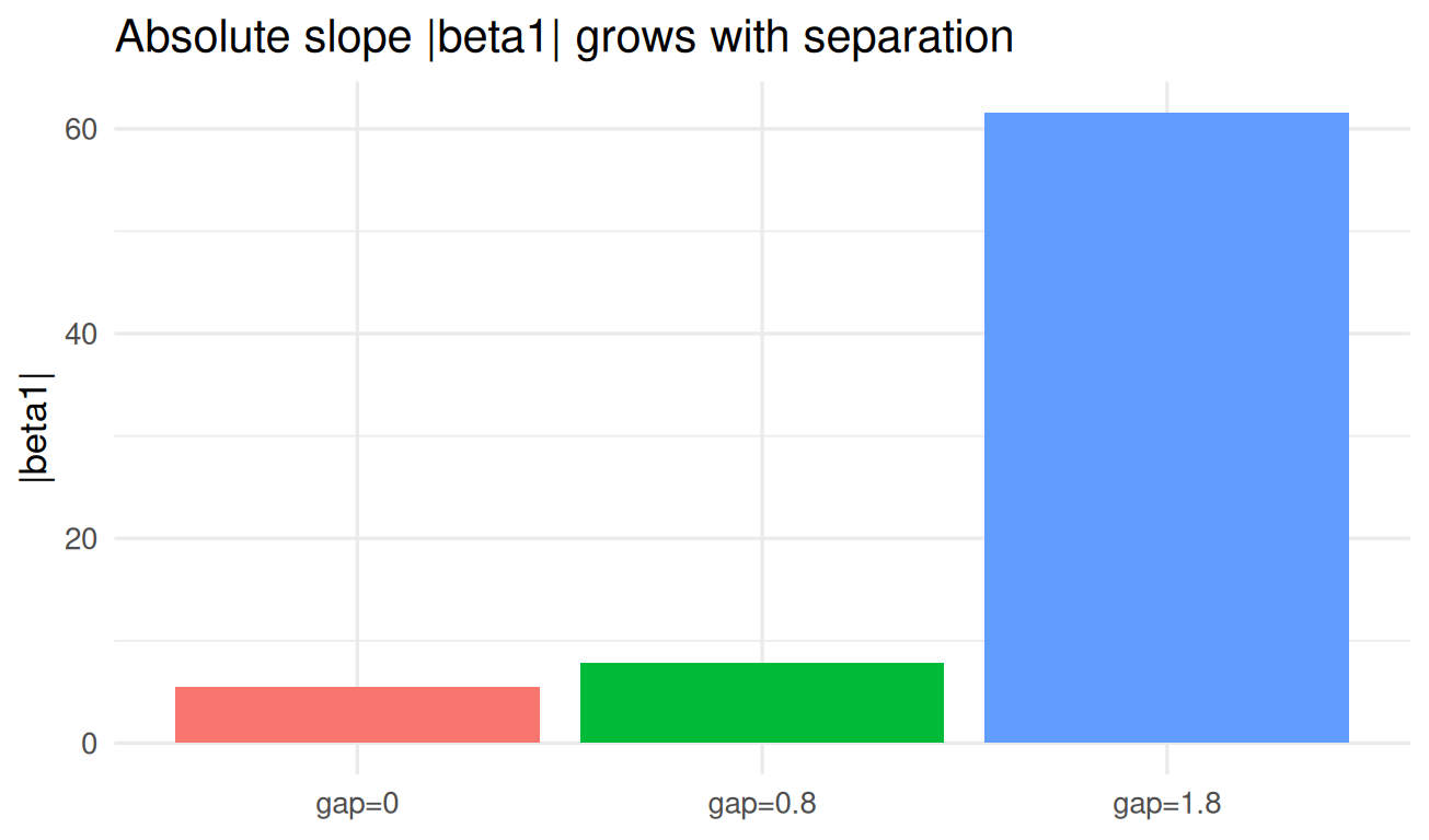
As classes become easier to separate on a single feature, the fitted slope \(\beta_1\) gets larger, so the S-curve becomes steeper. Under (near-)perfect separation, \(\beta_1\) can keep growing rather than settling to a stable finite value.
```{r one-d-separation}
set.seed(42)

make_1d <- function(gap = 0.0, n = 70) {
  x0 <- rnorm(n, mean = -0.7 - gap / 2, sd = 0.55)
  x1 <- rnorm(n, mean =  0.7 + gap / 2, sd = 0.55)
  tibble(
    x = c(x0, x1),
    y = factor(c(rep(0, n), rep(1, n)), levels = c(0, 1), labels = c("Class 0", "Class 1")),
    scenario = paste0("gap=", gap)
  )
}

d_small <- make_1d(gap = 0.0)
d_med   <- make_1d(gap = 0.8)
d_big   <- make_1d(gap = 1.8)
d_1d <- bind_rows(d_small, d_med, d_big)

fit_1d <- function(dat) glm(y ~ x, data = dat, family = binomial)
mods_1d <- d_1d |>
  group_split(scenario) |>
  setNames(unique(d_1d$scenario)) |>
  lapply(fit_1d)

coef_tbl <- tibble(
  scenario = names(mods_1d),
  intercept = sapply(mods_1d, \(m) coef(m)[1]),
  slope = sapply(mods_1d, \(m) coef(m)[2]),
  converged = sapply(mods_1d, \(m) m$converged)
)

coef_tbl
```
```{r one-d-curves, fig.width=9, fig.height=4.8}
grid_df <- d_1d |>
  group_by(scenario) |>
  summarize(x = list(seq(min(x) - 0.4, max(x) + 0.4, length.out = 250)), .groups = "drop") |>
  tidyr::unnest(x) |>
  group_by(scenario) |>
  mutate(
    p = predict(mods_1d[[first(scenario)]], newdata = cur_data(), type = "response")
  ) |>
  ungroup()

ggplot() +
  geom_jitter(
    data = d_1d,
    aes(x = x, y = as.numeric(y) - 1, color = y),
    height = 0.045,
    alpha = 0.35,
    size = 1.5
  ) +
  geom_line(
    data = grid_df,
    aes(x = x, y = p),
    linewidth = 1.1,
    color = "black"
  ) +
  facet_wrap(~scenario, nrow = 1) +
  scale_color_brewer(palette = "Set1") +
  scale_y_continuous(limits = c(-0.02, 1.02), breaks = c(0, 0.5, 1)) +
  labs(
    title = "1D logistic fit as separation increases",
    subtitle = "Fitted probability curve gets steeper as class gap increases",
    x = "Single predictor x",
    y = "P(Class 1)"
  )
```
```{r one-d-coef-plot, fig.width=6.8, fig.height=4}
ggplot(coef_tbl, aes(scenario, abs(slope), fill = scenario)) +
  geom_col(show.legend = FALSE) +
  labs(
    title = "Absolute slope |beta1| grows with separation",
    x = NULL,
    y = "|beta1|"
  )
```
## 2) Force a near-separated, high-dimensional situation
Here we deliberately create a bad setup to mirror what happens in wide microbiome tables:
1. add many noisy columns (`p` grows quickly), and
2. add one **leaky proxy** of the label (`leak`) that is almost the answer.
```{r bad-design}
set.seed(7)
p_noise <- 220
noise_mat <- matrix(rnorm(nrow(peng) * p_noise), nrow = nrow(peng))
colnames(noise_mat) <- paste0("noise_", seq_len(p_noise))

peng_bad <- bind_cols(
  peng,
  as.data.frame(noise_mat)
) |>
  mutate(
    # almost perfectly separates Gentoo from Adelie
    leak = ifelse(y == "Gentoo", 1, 0) + rnorm(n(), sd = 0.01)
  )

dim(peng_bad)
```
```{r glm-warning}
form_bad <- as.formula(
  paste("y ~", paste(setdiff(names(peng_bad), "y"), collapse = " + "))
)

warn_msg <- NULL
m_bad <- withCallingHandlers(
  glm(form_bad, data = peng_bad, family = binomial),
  warning = function(w) {
    warn_msg <<- conditionMessage(w)
    invokeRestart("muffleWarning")
  }
)

list(
  converged = m_bad$converged,
  warning = warn_msg
)
```
```{r probs}
phat_bad <- predict(m_bad, type = "response")

tibble(
  min_p = min(phat_bad),
  p01 = mean(phat_bad < 0.01),
  p99 = mean(phat_bad > 0.99),
  max_p = max(phat_bad)
)
```
When probabilities bunch up at extremes and the optimizer struggles, the model is effectively trying to push coefficients toward very large values.
## 3) Why lasso is more stable
Lasso (`glmnet`) adds a penalty that keeps coefficients finite and controls overfitting.
```{r lasso}
x <- model.matrix(y ~ . - 1, data = peng_bad)
y01 <- ifelse(peng_bad$y == "Gentoo", 1, 0)

set.seed(7)
cv_lasso <- cv.glmnet(x, y01, family = "binomial", alpha = 1, nfolds = 5)

coef_lasso <- coef(cv_lasso, s = "lambda.min")
n_nonzero <- sum(coef_lasso != 0) - 1
n_nonzero
```
```{r compare-train}
pred_bad <- factor(ifelse(phat_bad > 0.5, "Gentoo", "Adelie"), levels = levels(peng_bad$y))
acc_bad <- mean(pred_bad == peng_bad$y)

phat_lasso <- as.numeric(predict(cv_lasso, newx = x, s = "lambda.min", type = "response"))
pred_lasso <- factor(ifelse(phat_lasso > 0.5, "Gentoo", "Adelie"), levels = levels(peng_bad$y))
acc_lasso <- mean(pred_lasso == peng_bad$y)

tibble(
  model = c("Unpenalized glm", "Lasso (glmnet)"),
  train_accuracy = c(acc_bad, acc_lasso)
)
```
## Take-home message
- With limited `n` and many predictors, unpenalized logistic regression can hit **(quasi-)separation**.
- Then coefficient estimates become unstable, probabilities saturate near `0/1`, and convergence warnings appear.
- Penalized models (lasso/ridge/elastic net) are usually safer in high-dimensional settings.