set.seed(7)
mic <- load_microbiome()
otu_cols <- mic_otu_cols(mic)

rec <- recipe(Label ~ ., data = mic) |>
  update_role(sample_id, Individual, Sex, Day, new_role = "id") |>
  step_mutate(across(all_of(otu_cols), ~ log1p(.x))) |>
  step_zv(all_predictors()) |>
  step_normalize(all_numeric_predictors())

folds <- mic_group_folds(mic, v = 5)
metrics_cls <- metric_set(roc_auc, accuracy)Solution — Day 4 microbiome (models + VIP + SHAP)
Tasks 4.1–4.5 on the lab exercises page.
4.1 Recipe
4.2 Fit RF, XGBoost, MLP
rf_spec <- rand_forest(mtry = 8, trees = 300, min_n = 2) |>
  set_engine("ranger", probability = TRUE, importance = "impurity") |>
  set_mode("classification")
xgb_spec <- boost_tree(trees = 100, tree_depth = 3, learn_rate = 0.05) |>
  set_engine("xgboost") |> set_mode("classification")
mlp_spec <- mlp(hidden_units = 10, penalty = 0.1, epochs = 150) |>
  set_engine("nnet", trace = FALSE, MaxNWts = 5000) |> set_mode("classification")
# Grouped CV on ~300 OTUs is the slowest step (~1–3 min). Cached after first knit.
set.seed(7)
rs_rf <- fit_resamples(workflow() |> add_recipe(rec) |> add_model(rf_spec), folds, metrics_cls)
set.seed(7)
rs_xgb <- fit_resamples(workflow() |> add_recipe(rec) |> add_model(xgb_spec), folds, metrics_cls)
set.seed(9)
rs_mlp <- fit_resamples(workflow() |> add_recipe(rec) |> add_model(mlp_spec), folds, metrics_cls)
cmp <- bind_rows(
collect_metrics(rs_rf) |> mutate(model = "Random forest"),
collect_metrics(rs_xgb) |> mutate(model = "XGBoost"),
collect_metrics(rs_mlp) |> mutate(model = "MLP")
)
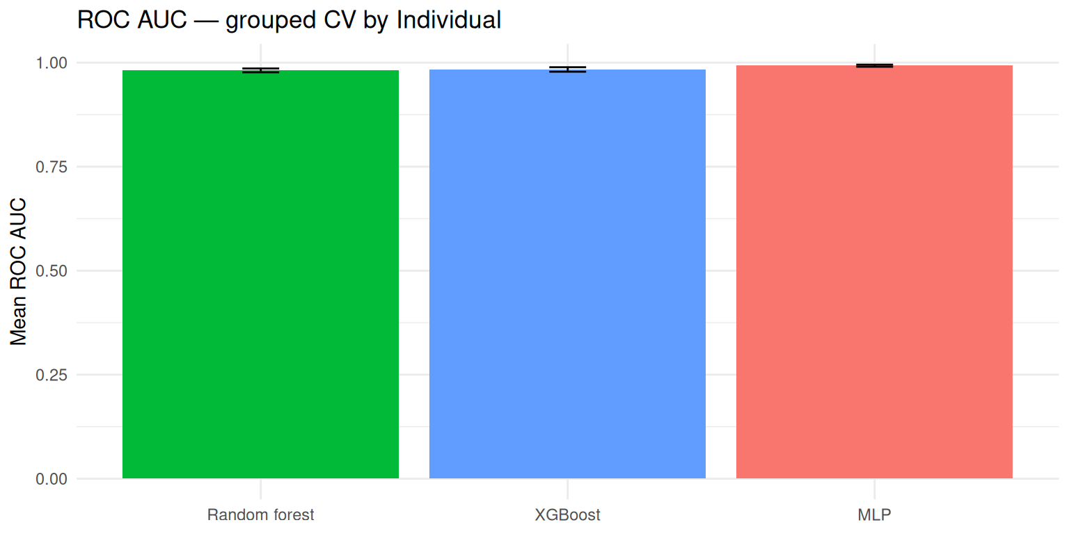
knitr::kable(cmp |> filter(.metric == "roc_auc") |> select(model, mean, std_err), digits = 3)| model | mean | std_err |
|---|---|---|
| Random forest | 0.981 | 0.005 |
| XGBoost | 0.984 | 0.005 |
| MLP | 0.993 | 0.002 |
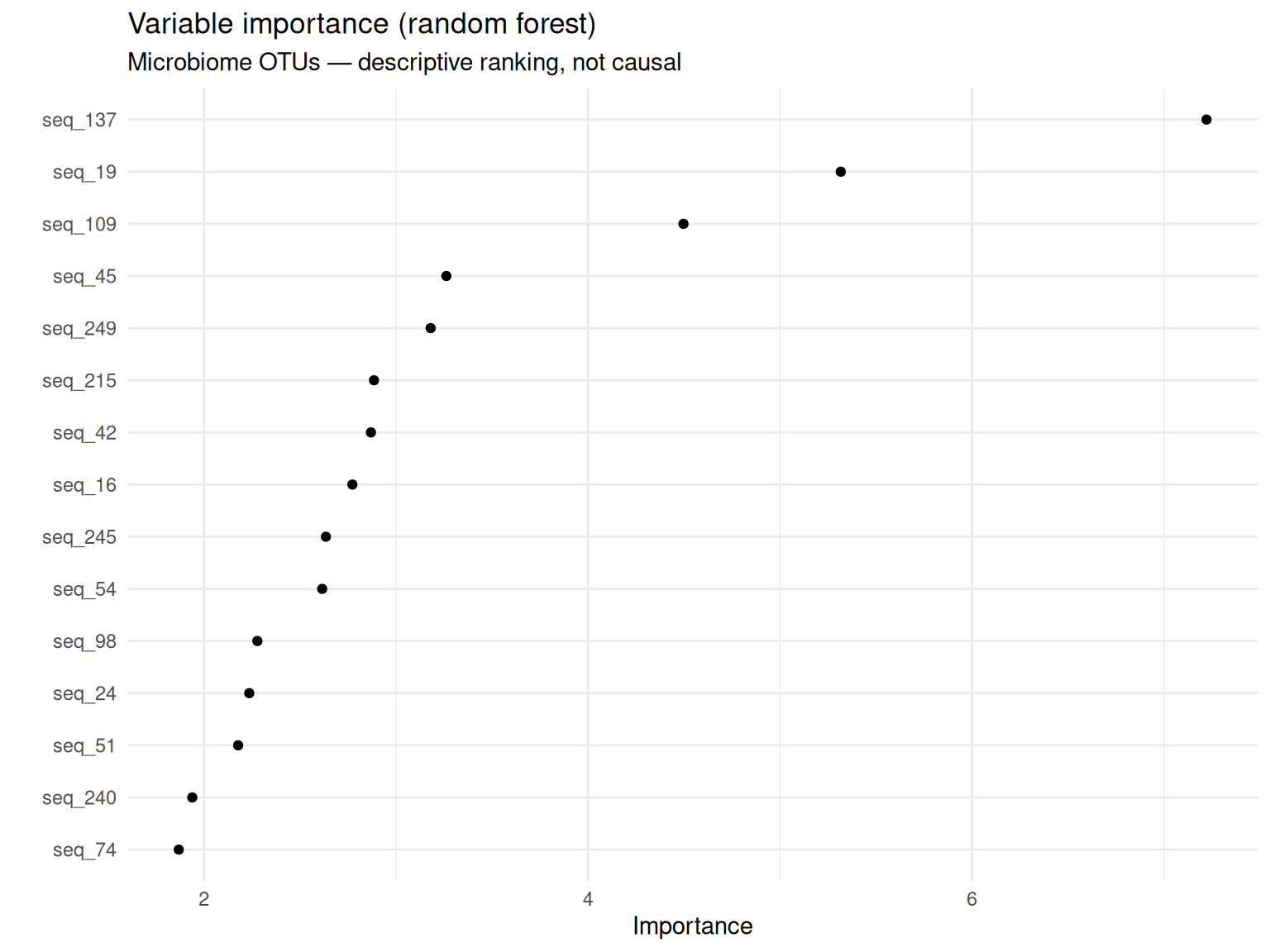
4.3 VIP (random forest)
wf_rf <- workflow() |> add_recipe(rec) |> add_model(rf_spec)
fit_rf <- fit(wf_rf, mic)
fit_rf |>
extract_fit_parsnip() |>
vip(geom = "point", num_features = 15) +
labs(
title = "Variable importance (random forest)",
subtitle = "Microbiome OTUs — descriptive ranking, not causal"
)
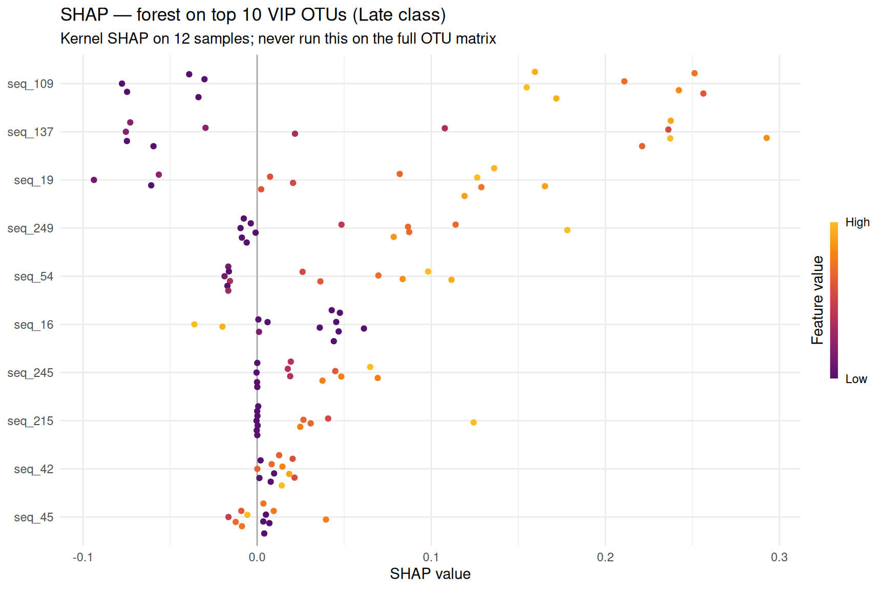
4.4 SHAP
Do not run kernel SHAP on all OTUs — with 300+ predictors it can run for hours. We take the top 10 VIP OTUs, refit a small forest for teaching, and explain 12 samples (same pattern as the penguin SHAP slides, fewer features).
vip_top <- vip::vi(extract_fit_parsnip(fit_rf)) |>
  arrange(desc(Importance)) |>
  slice_head(n = 10) |>
  pull(Variable)

mic_top <- mic |> select(Label, sample_id, Individual, Sex, Day, all_of(vip_top))
rec_top <- recipe(Label ~ ., data = mic_top) |>
update_role(sample_id, Individual, Sex, Day, new_role = "id") |>
step_mutate(across(all_of(vip_top), ~ log1p(.x))) |>
step_zv(all_predictors()) |>
step_normalize(all_numeric_predictors())
rf_top_spec <- rand_forest(mtry = 3, trees = 100, min_n = 2) |>
set_engine("ranger", probability = TRUE) |>
set_mode("classification")
fit_rf_top <- fit(
workflow() |> add_recipe(rec_top) |> add_model(rf_top_spec),
mic_top
)if (requireNamespace("kernelshap", quietly = TRUE)) {
options(kernelshap.verbose = FALSE)
}
rec_est <- extract_recipe(fit_rf_top, estimated = TRUE)
X_model <- bake(rec_est, new_data = mic_top, all_predictors())
rf_engine <- extract_fit_parsnip(fit_rf_top)$fit
pred_fun <- function(object, X_new) {
as.numeric(predict(object, data = X_new)$predictions[, "Late"])
}
set.seed(11)
n_explain <- min(12L, nrow(X_model))
n_bg <- min(6L, nrow(X_model))
X <- X_model[sample.int(nrow(X_model), n_explain), , drop = FALSE]
bg <- dplyr::slice_sample(X_model, n = n_bg)
ks <- kernelshap::kernelshap(rf_engine, X = X, pred_fun = pred_fun, bg_X = bg)
  |
  |                                                                      |   0%
  |
  |======                                                                |   8%
  |
  |============                                                          |  17%
  |
  |==================                                                    |  25%
  |
  |=======================                                               |  33%
  |
  |=============================                                         |  42%
  |
  |===================================                                   |  50%
  |
  |=========================================                             |  58%
  |
  |===============================================                       |  67%
  |
  |====================================================                  |  75%
  |
  |==========================================================            |  83%
  |
  |================================================================      |  92%
  |
  |======================================================================| 100%
shp <- shapviz::shapviz(ks, X_pred = X)sv_importance(shp, kind = "beeswarm", max_display = 12) +
labs(
title = "SHAP — forest on top 10 VIP OTUs (Late class)",
subtitle = "Kernel SHAP on 12 samples; never run this on the full OTU matrix"
)
4.5 Comparison figure
cmp |>
  filter(.metric == "roc_auc") |>
  ggplot(aes(reorder(model, mean), mean, fill = model)) +
  geom_col(show.legend = FALSE) +
  geom_errorbar(aes(ymin = mean - std_err, ymax = mean + std_err), width = 0.12) +
  labs(
    title = "ROC AUC — grouped CV by Individual",
    x = NULL, y = "Mean ROC AUC"
  )
Humility: I would not claim that the top VIP or SHAP OTU causes Early vs Late community shift — these plots describe this fitted model on observational counts, not a randomized intervention.
R version 4.4.3 (2025-02-28)
Platform: x86_64-pc-linux-gnu
Running under: Ubuntu 24.04.4 LTS

Matrix products: default
BLAS:   /usr/lib/x86_64-linux-gnu/openblas-pthread/libblas.so.3
LAPACK: /usr/lib/x86_64-linux-gnu/openblas-pthread/libopenblasp-r0.3.26.so;  LAPACK version 3.12.0

locale:
 [1] LC_CTYPE=C.UTF-8       LC_NUMERIC=C           LC_TIME=C.UTF-8
 [4] LC_COLLATE=C.UTF-8     LC_MONETARY=C.UTF-8    LC_MESSAGES=C.UTF-8
 [7] LC_PAPER=C.UTF-8       LC_NAME=C              LC_ADDRESS=C
[10] LC_TELEPHONE=C         LC_MEASUREMENT=C.UTF-8 LC_IDENTIFICATION=C

time zone: UTC
tzcode source: system (glibc)

attached base packages:
[1] stats     graphics  grDevices utils     datasets  methods   base

other attached packages:
 [1] shapviz_0.10.3     kernelshap_0.9.1   vip_0.4.6          yardstick_1.4.0
 [5] workflowsets_1.1.1 workflows_1.3.0    tune_2.1.0         tidyr_1.3.2
 [9] tailor_0.1.0       rsample_1.3.2      recipes_1.3.3      purrr_1.2.2
[13] parsnip_1.6.0      modeldata_1.5.1    infer_1.1.0        ggplot2_4.0.3
[17] dplyr_1.2.1        dials_1.4.3        scales_1.4.0       broom_1.0.13
[21] tidymodels_1.5.0

loaded via a namespace (and not attached):
 [1] tidyselect_1.2.1    viridisLite_0.4.3   timeDate_4052.112
 [4] farver_2.1.2        S7_0.2.2            fastmap_1.2.0
 [7] digest_0.6.39       rpart_4.1.24        timechange_0.4.0
[10] lifecycle_1.0.5     survival_3.8-3      magrittr_2.0.5
[13] compiler_4.4.3      rlang_1.2.0         tools_4.4.3
[16] yaml_2.3.12         data.table_1.18.4   knitr_1.51
[19] labeling_0.4.3      curl_7.1.0          bit_4.6.0
[22] xgboost_3.2.1.1     DiceDesign_1.10     RColorBrewer_1.1-3
[25] withr_3.0.2         nnet_7.3-20         grid_4.4.3
[28] sparsevctrs_0.3.6   future_1.70.0       globals_0.19.1
[31] iterators_1.0.14    MASS_7.3-64         cli_3.6.6
[34] crayon_1.5.3        rmarkdown_2.31      generics_0.1.4
[37] otel_0.2.0          rstudioapi_0.18.0   future.apply_1.20.2
[40] tzdb_0.5.0          splines_4.4.3       parallel_4.4.3
[43] vctrs_0.7.3         hardhat_1.4.3       Matrix_1.7-2
[46] jsonlite_2.0.0      hms_1.1.4           bit64_4.8.2
[49] listenv_0.10.1      foreach_1.5.2       gower_1.0.2
[52] glue_1.8.1          parallelly_1.47.0   codetools_0.2-20
[55] lubridate_1.9.5     gtable_0.3.6        doFuture_1.2.2
[58] tibble_3.3.1        pillar_1.11.1       furrr_0.4.0
[61] htmltools_0.5.9     ipred_0.9-15        lava_1.9.1
[64] R6_2.6.1            vroom_1.7.1         evaluate_1.0.5
[67] lattice_0.22-6      readr_2.2.0         backports_1.5.1
[70] class_7.3-23        Rcpp_1.1.1-1.1      prodlim_2026.03.11
[73] ranger_0.18.0       xfun_0.58           pkgconfig_2.0.3