source("_load_microbiome.R")

# One metric only — pass this to last_fit(), tune_grid(), etc.
accuracy_only <- metric_set(accuracy)Solution — Day 2 microbiome (tidymodels pipeline)
Tasks 2.1–2.5 on the lab exercises page. Outcome: Label (Early vs Late). We use accuracy throughout and compare rpart, unpenalized logistic regression (glm), and lasso (glmnet) on the same train/test split.
Microbiome helpers (load_microbiome(), mic_otu_cols(), …) live in _load_microbiome.R on GitHub. When you run this file locally, source() it from exercises/solutions/.
New to tidymodels? Use the companion explainer: Day 2 function guide (plain language).
2.1 Recipe
set.seed(7)
mic <- load_microbiome()
otu_cols <- mic_otu_cols(mic)
mic_model <- mic |> select(Label, all_of(otu_cols))

table(mic_model$Label)
Early  Late
  177   105
rec <- recipe(Label ~ ., data = mic_model) |>
step_mutate(across(all_of(otu_cols), ~ log1p(.x))) |>
step_zv(all_predictors()) |>
step_normalize(all_numeric_predictors())
rec2.2 rpart tree spec
tree_spec <- decision_tree(tree_depth = 4, min_n = 10) |>
  set_engine("rpart") |>
  set_mode("classification")
tree_spec
Decision Tree Model Specification (classification)
Main Arguments:
tree_depth = 4
min_n = 10
Computational engine: rpart 2.3 Train / test split
We hold out 25% of rows for a stratified test set. The recipe is prepped on training rows only when we fit() — that is the leakage-safe pattern from the slides.
split <- initial_split(mic_model, prop = 0.75, strata = Label)
train <- training(split)
test <- testing(split)

tibble(
  set = c("Train", "Test"),
  n = c(nrow(train), nrow(test)),
  pct_late = c(mean(train$Label == "Late"), mean(test$Label == "Late"))
) |>
knitr::kable(digits = 3, caption = "Split sizes and Late prevalence")| set | n | pct_late |
|---|---|---|
| Train | 210 | 0.371 |
| Test | 72 | 0.375 |
bind_rows(
  train |> mutate(set = "Train"),
  test |> mutate(set = "Test")
) |>
  ggplot(aes(set, fill = Label)) +
  geom_bar(position = "fill") +
  scale_y_continuous(labels = scales::percent_format()) +
  scale_fill_brewer(palette = "Set2") +
  labs(title = "Class balance in train vs test", x = NULL, y = "Proportion")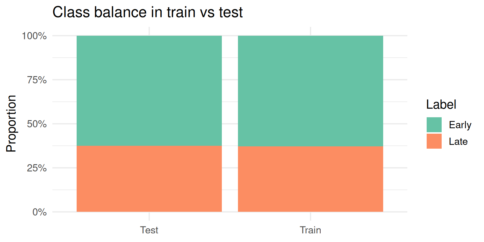
wf_tree <- workflow() |> add_recipe(rec) |> add_model(tree_spec)set.seed(7)
fit_tree <- last_fit(wf_tree, split, metrics = accuracy_only)
collect_metrics(fit_tree)# A tibble: 1 × 4
.metric .estimator .estimate .config
<chr> <chr> <dbl> <chr>
1 accuracy binary 0.931 pre0_mod0_post0set.seed(7)
fitted_tree <- fit(wf_tree, train)
pred_tree_train <- augment(fitted_tree, train)
pred_tree_test <- augment(fitted_tree, test)
accuracy(pred_tree_train, truth = Label, estimate = .pred_class)# A tibble: 1 × 3
.metric .estimator .estimate
<chr> <chr> <dbl>
1 accuracy binary 0.981accuracy(pred_tree_test, truth = Label, estimate = .pred_class)# A tibble: 1 × 3
.metric .estimator .estimate
<chr> <chr> <dbl>
1 accuracy binary 0.9312.4 Logistic regression (unpenalized glm)
log_spec <- logistic_reg() |>
  set_engine("glm") |>
  set_mode("classification")
wf_log <- workflow() |> add_recipe(rec) |> add_model(log_spec)set.seed(7)
fit_log <- last_fit(wf_log, split, metrics = accuracy_only)
collect_metrics(fit_log)# A tibble: 1 × 4
.metric .estimator .estimate .config
<chr> <chr> <dbl> <chr>
1 accuracy binary 0.431 pre0_mod0_post0Fit on the training set so we can score train and test explicitly with yardstick::accuracy():
set.seed(7)
fitted_log <- fit(wf_log, train)
pred_train <- augment(fitted_log, train)
pred_test <- augment(fitted_log, test)

# yardstick::accuracy() — truth and estimate column names must match
accuracy(pred_train, truth = Label, estimate = .pred_class)
# A tibble: 1 × 3
.metric .estimator .estimate
<chr> <chr> <dbl>
1 accuracy binary 1accuracy(pred_test, truth = Label, estimate = .pred_class)# A tibble: 1 × 3
.metric .estimator .estimate
<chr> <chr> <dbl>
1 accuracy binary 0.4312.5 Lasso logistic regression (glmnet)
Same recipe, but mixture = 1 is lasso and penalty (λ) is tuned by 5-fold CV on the training set only — the Day 1 idea inside a tidymodels workflow.
lasso_spec <- logistic_reg(penalty = tune(), mixture = 1) |>
  set_engine("glmnet") |>
  set_mode("classification")
wf_lasso <- workflow() |> add_recipe(rec) |> add_model(lasso_spec)set.seed(7)
folds <- vfold_cv(train, v = 5, strata = Label)
grid <- grid_regular(penalty(range = c(-4, 0)), levels = 10)
tuned_lasso <- tune_grid(
wf_lasso,
resamples = folds,
grid = grid,
metrics = accuracy_only
)
select_best(tuned_lasso, metric = "accuracy")# A tibble: 1 × 2
penalty .config
<dbl> <chr>
1 0.0001 pre0_mod01_post0wf_lasso_final <- finalize_workflow(wf_lasso, select_best(tuned_lasso, metric = "accuracy"))
set.seed(7)
fit_lasso <- last_fit(wf_lasso_final, split, metrics = accuracy_only)
collect_metrics(fit_lasso)# A tibble: 1 × 4
.metric .estimator .estimate .config
<chr> <chr> <dbl> <chr>
1 accuracy binary 0.986 pre0_mod0_post02.6 Compare models on the test set (accuracy)
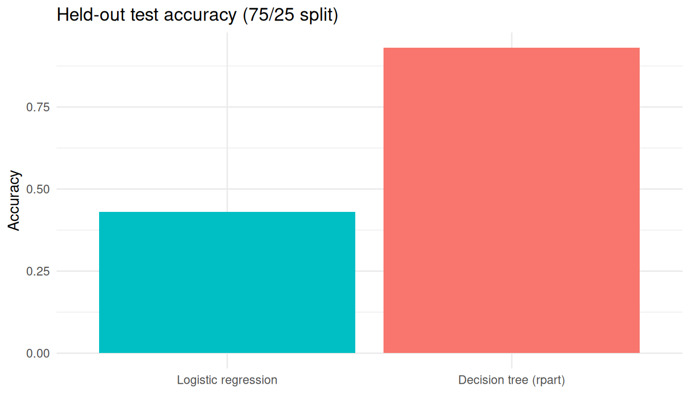
All three models use the same split and recipe. last_fit() fits on training(split) and reports accuracy on testing(split):
cmp <- bind_rows(
  collect_metrics(fit_tree) |> mutate(model = "rpart (tree)"),
  collect_metrics(fit_log) |> mutate(model = "Logistic (glm)"),
  collect_metrics(fit_lasso) |> mutate(model = "Lasso (glmnet)")
) |>
  select(model, .metric, .estimate)

majority_acc <- max(prop.table(table(test$Label)))

cmp |>
  bind_rows(tibble(model = "Majority class", .metric = "accuracy", .estimate = majority_acc)) |>
knitr::kable(digits = 3, caption = "Held-out test accuracy (75/25 split)")| model | .metric | .estimate |
|---|---|---|
| rpart (tree) | accuracy | 0.931 |
| Logistic (glm) | accuracy | 0.431 |
| Lasso (glmnet) | accuracy | 0.986 |
| Majority class | accuracy | 0.625 |
cmp |>
  ggplot(aes(reorder(model, .estimate), .estimate, fill = model)) +
  geom_col(show.legend = FALSE) +
  geom_hline(yintercept = majority_acc, linetype = 2, linewidth = 0.7) +
  coord_flip() +
  labs(
    title = "Test accuracy — rpart vs glm vs lasso",
    subtitle = "Dashed line = majority-class baseline on the test set",
    x = NULL,
    y = "Accuracy"
  )
2.7 Train vs test accuracy — all three models
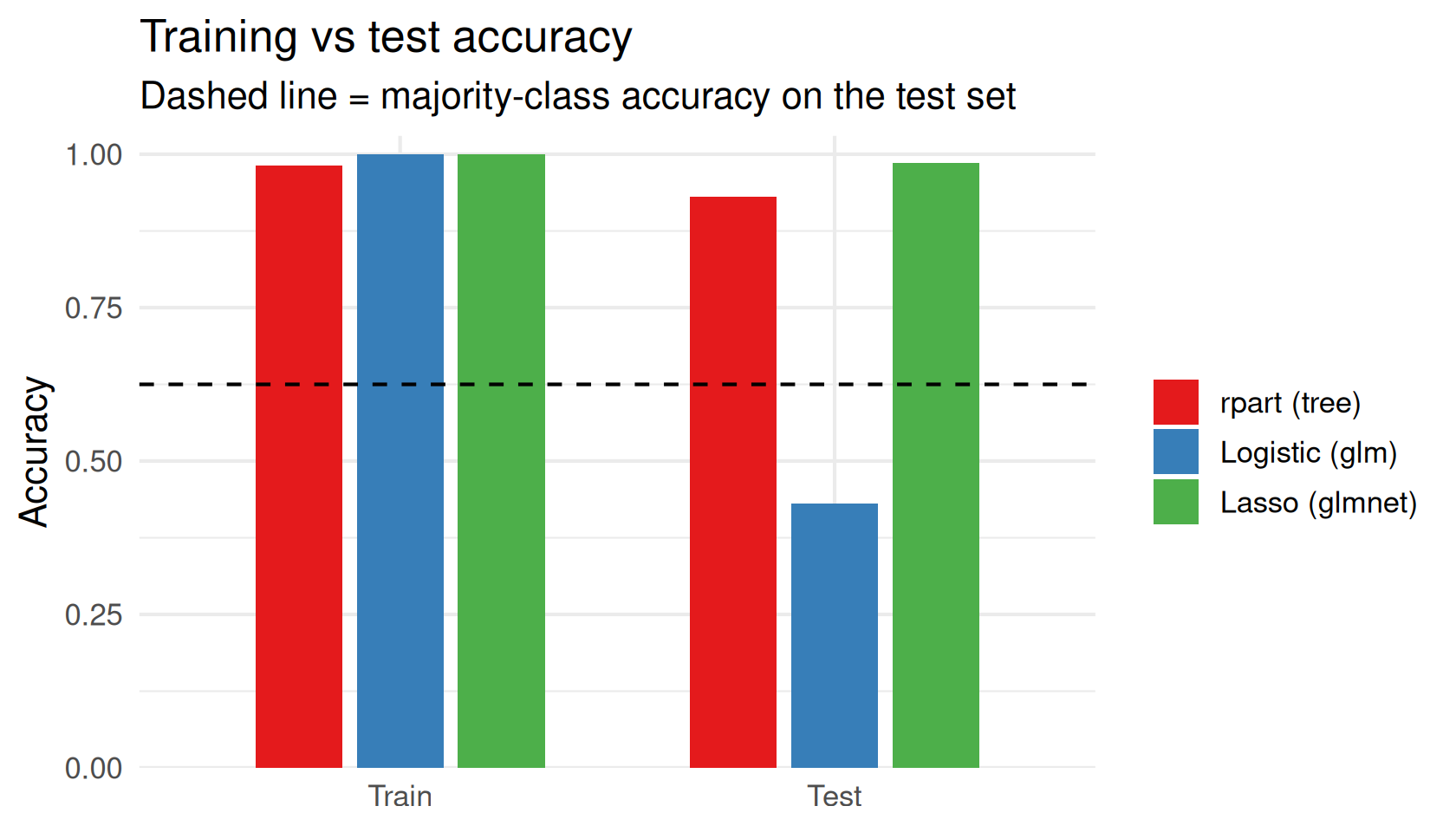
Unpenalized logistic regression has more OTU predictors than training samples (344 OTUs, 210 train rows). glm may not converge and can achieve perfect training accuracy while doing worse than the majority class on the test set. rpart and lasso handle high-dimensional predictors more safely (splits vs penalised coefficients).
fitted_lasso <- fit(wf_lasso_final, train)
pred_lasso_train <- augment(fitted_lasso, train)
pred_lasso_test <- augment(fitted_lasso, test)

acc_value <- function(df) {
  accuracy(df, truth = Label, estimate = .pred_class)$.estimate
}

acc_tbl <- tibble(
  model = rep(c("rpart (tree)", "Logistic (glm)", "Lasso (glmnet)"), each = 2),
  set = rep(c("Train", "Test"), times = 3),
  accuracy = c(
    acc_value(pred_tree_train), acc_value(pred_tree_test),
    acc_value(pred_train), acc_value(pred_test),
    acc_value(pred_lasso_train), acc_value(pred_lasso_test)
  )
)

knitr::kable(acc_tbl, digits = 3, caption = "Accuracy via yardstick::accuracy()")| model | set | accuracy |
|---|---|---|
| rpart (tree) | Train | 0.981 |
| rpart (tree) | Test | 0.931 |
| Logistic (glm) | Train | 1.000 |
| Logistic (glm) | Test | 0.431 |
| Lasso (glmnet) | Train | 1.000 |
| Lasso (glmnet) | Test | 0.986 |
acc_tbl |>
  mutate(
    model = factor(
      model,
      levels = c("rpart (tree)", "Logistic (glm)", "Lasso (glmnet)")
    ),
    set = factor(set, levels = c("Train", "Test"))
  ) |>
  ggplot(aes(set, accuracy, fill = model)) +
  geom_col(position = position_dodge(width = 0.7), width = 0.6) +
  geom_hline(yintercept = majority_acc, linetype = 2) +
  scale_fill_brewer(palette = "Set1") +
  scale_y_continuous(limits = c(0, 1), expand = expansion(mult = c(0, 0.03))) +
  labs(
    title = "Training vs test accuracy",
    subtitle = "Dashed line = majority-class accuracy on the test set",
    x = NULL,
    y = "Accuracy",
    fill = NULL
  )
conf_to_df <- function(x, model) {
  as.data.frame(x$table) |>
    mutate(model = model)
}

bind_rows(
  conf_to_df(conf_mat(pred_tree_test, truth = Label, estimate = .pred_class), "rpart (tree)"),
  conf_to_df(conf_mat(pred_test, truth = Label, estimate = .pred_class), "Logistic (glm)"),
  conf_to_df(conf_mat(pred_lasso_test, truth = Label, estimate = .pred_class), "Lasso (glmnet)")
) |>
  ggplot(aes(Prediction, Truth, fill = Freq)) +
  geom_tile(color = "white") +
  geom_text(aes(label = Freq), color = "white", fontface = "bold") +
  facet_wrap(~ model) +
  scale_fill_gradient(low = "grey85", high = "steelblue") +
  labs(title = "Test-set confusion matrices", x = "Predicted", y = "Observed")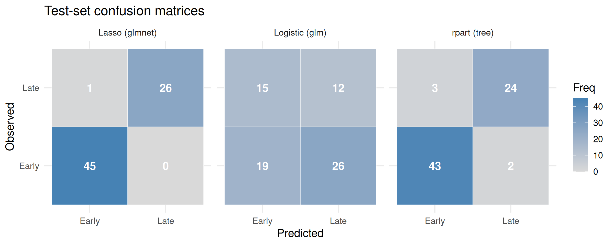
Takeaways
- Specify the metric:
accuracy_only <- metric_set(accuracy)for resampling;accuracy(data, truth = Label, estimate = .pred_class)on prediction tables. - Unpenalized glm + p ≫ n → unreliable test accuracy;
rpartand lasso are safer choices on the same OTU matrix. rpartuses recursive splits (morning Part B); lasso uses penalised coefficients (Monday’sglmnet, now in a workflow).- Repeated measures:
initial_split()can put the same mouse in train and test; Day 4 usesgroup_vfold_cv(group = Individual).
Leakage reminder: prep the recipe inside fit() / workflow on training data only; never normalize on the full table before splitting.
R version 4.4.3 (2025-02-28)
Platform: x86_64-pc-linux-gnu
Running under: Ubuntu 24.04.4 LTS

Matrix products: default
BLAS:   /usr/lib/x86_64-linux-gnu/openblas-pthread/libblas.so.3
LAPACK: /usr/lib/x86_64-linux-gnu/openblas-pthread/libopenblasp-r0.3.26.so;  LAPACK version 3.12.0

locale:
 [1] LC_CTYPE=C.UTF-8       LC_NUMERIC=C           LC_TIME=C.UTF-8
 [4] LC_COLLATE=C.UTF-8     LC_MONETARY=C.UTF-8    LC_MESSAGES=C.UTF-8
 [7] LC_PAPER=C.UTF-8       LC_NAME=C              LC_ADDRESS=C
[10] LC_TELEPHONE=C         LC_MEASUREMENT=C.UTF-8 LC_IDENTIFICATION=C

time zone: UTC
tzcode source: system (glibc)

attached base packages:
[1] stats     graphics  grDevices utils     datasets  methods   base

other attached packages:
 [1] patchwork_1.3.2    yardstick_1.4.0    workflowsets_1.1.1 workflows_1.3.0
 [5] tune_2.1.0         tidyr_1.3.2        tailor_0.1.0       rsample_1.3.2
 [9] recipes_1.3.3      purrr_1.2.2        parsnip_1.6.0      modeldata_1.5.1
[13] infer_1.1.0        ggplot2_4.0.3      dplyr_1.2.1        dials_1.4.3
[17] scales_1.4.0       broom_1.0.13       tidymodels_1.5.0

loaded via a namespace (and not attached):
 [1] tidyselect_1.2.1    timeDate_4052.112   farver_2.1.2
 [4] S7_0.2.2            fastmap_1.2.0       digest_0.6.39
 [7] rpart_4.1.24        timechange_0.4.0    lifecycle_1.0.5
[10] survival_3.8-3      magrittr_2.0.5      compiler_4.4.3
[13] rlang_1.2.0         tools_4.4.3         utf8_1.2.6
[16] yaml_2.3.12         data.table_1.18.4   knitr_1.51
[19] labeling_0.4.3      curl_7.1.0          bit_4.6.0
[22] DiceDesign_1.10     RColorBrewer_1.1-3  withr_3.0.2
[25] nnet_7.3-20         grid_4.4.3          sparsevctrs_0.3.6
[28] future_1.70.0       iterators_1.0.14    globals_0.19.1
[31] MASS_7.3-64         cli_3.6.6           crayon_1.5.3
[34] rmarkdown_2.31      generics_0.1.4      otel_0.2.0
[37] rstudioapi_0.19.0   future.apply_1.20.2 tzdb_0.5.0
[40] splines_4.4.3       parallel_4.4.3      vctrs_0.7.3
[43] glmnet_5.0          hardhat_1.4.3       Matrix_1.7-2
[46] jsonlite_2.0.0      hms_1.1.4           bit64_4.8.2
[49] listenv_0.10.1      foreach_1.5.2       gower_1.0.2
[52] glue_1.8.1          parallelly_1.47.0   codetools_0.2-20
[55] shape_1.4.6.1       lubridate_1.9.5     gtable_0.3.6
[58] tibble_3.3.1        pillar_1.11.1       furrr_0.4.0
[61] htmltools_0.5.9     ipred_0.9-15        lava_1.9.1
[64] R6_2.6.1            vroom_1.7.1         evaluate_1.0.5
[67] lattice_0.22-6      readr_2.2.0         backports_1.5.1
[70] class_7.3-23        Rcpp_1.1.1-1.1      prodlim_2026.03.11
[73] xfun_0.58           pkgconfig_2.0.3