In this post we are going to explore the likelihood, the log-likelihood and how to derive a maximum likelihood estimator for the parameters of a Poisson distribution.
We start by genearting a random data set:
set.seed(42)
sample.size = 100
lambda = 2
x = rpois(sample.size,lambda)
This is a sample from a Poisson distribution, with mean \(\lambda =2\). We sinterpret it as i.i.d. realizations of a random variable \(X\) and label the data points: \(x_1, x_2, \ldots, x_n\), where n is the sample size.
For a given pqrameter \(\lambda\), the probabiltiy to observe the value \(x \in \{ 0,1,2,3, ... \}\) is given by: \(e^{-\lambda} \frac{\lambda^{x}}{x!}\). The likelihood of the sample is the the joint probability mass function of the whole sample as a function of the parameter \(\lambda\). Becassue the data points are independent, the likelihood is then simply the product of the individual probabilties for each \(x_i\): \[\displaystyle L(\lambda) = \prod_{i=1}^n e^{-\lambda} \frac{\lambda^{x_i}}{x_i!}.\]
We can plot this for our example:
lambda.vec = seq(1,3,by = 0.01)
L = 1
for(i in 1: sample.size)
{
  L = L*dpois(x[i],lambda.vec)
}

dat = data.frame(lambda = lambda.vec,Likelihood = L)


ggplot(data = dat,aes(x = lambda,y= Likelihood)) +
  geom_line() +
  theme(text = element_text(size = 20)) +
theme_classic() 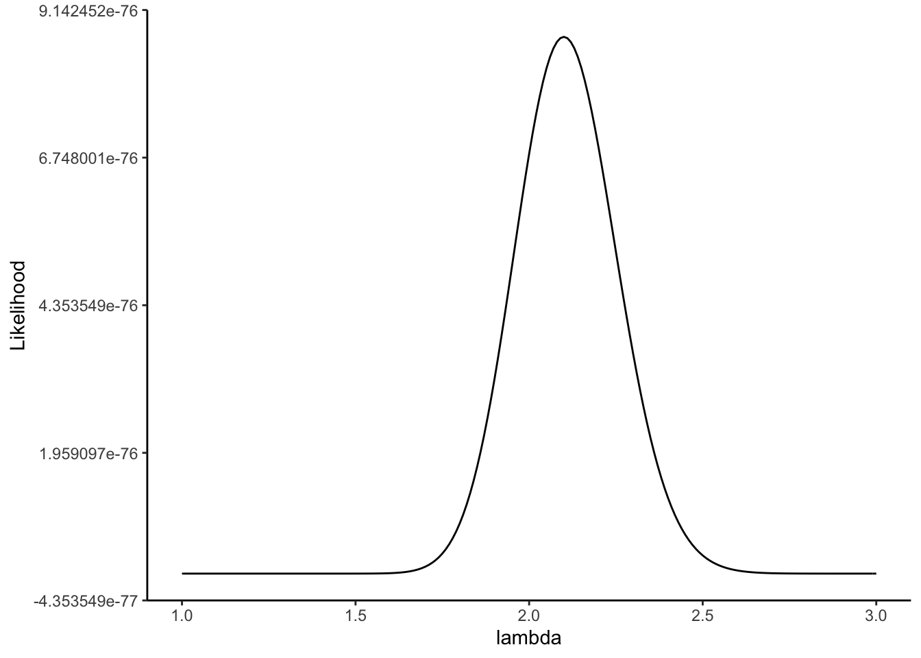
Next we plot the log-likelihood of the sample: \[\displaystyle \ell(\lambda) = \sum_{i=1}^n \left[ x_i \log(\lambda) - \lambda - \log(x_i!) \right]\]
ggplot(data = dat,aes(x = lambda,y= log(Likelihood))) +
  geom_line() +
  theme(text = element_text(size = 20)) +
theme_classic() 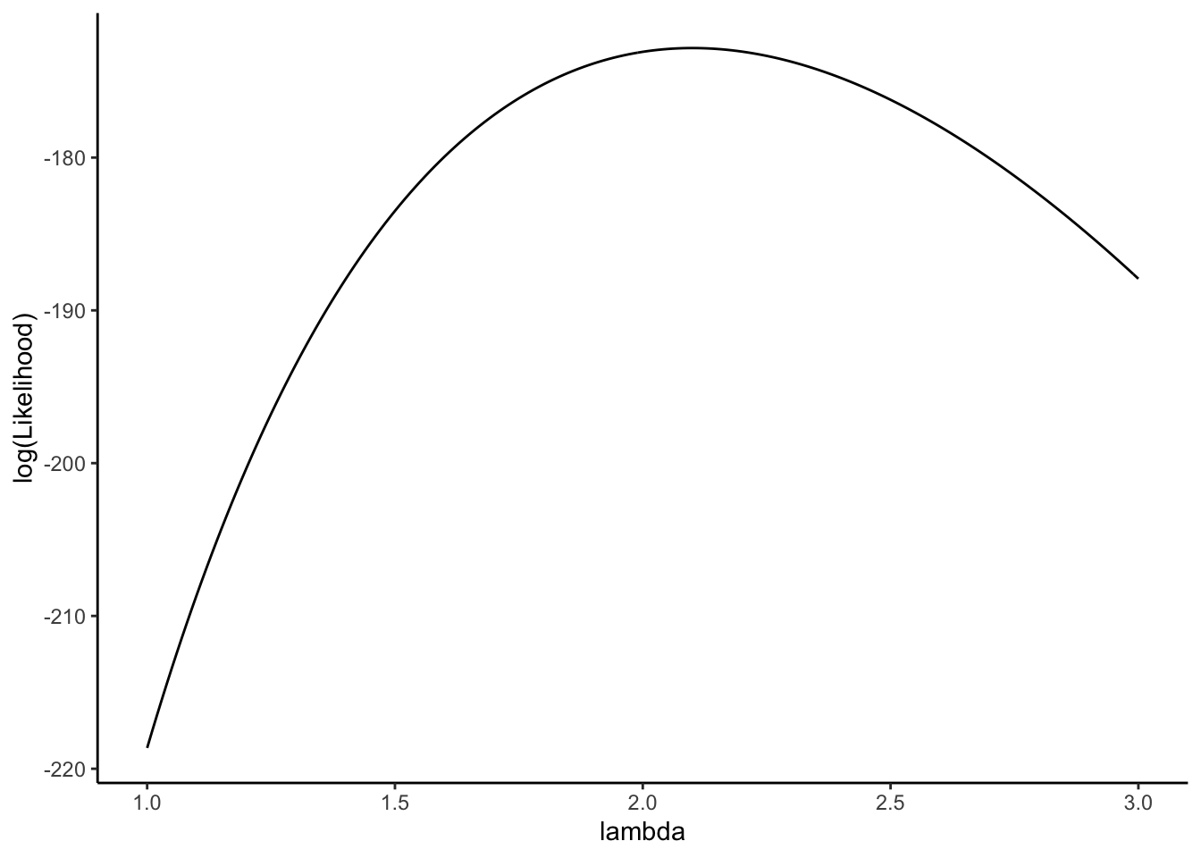
Note that the log likelihood and the likelihood are maximized for the same value of \(\lambda\)!
Finally we are going to derive the maximum likelihood estimator. It is much simpler to do this for the log-likelihood. First we take the derivateive with respect to \(\lambda:\)
\[\frac{d} {d\lambda}\displaystyle \ell(\lambda) = \sum_{i=1}^n \left[ x_i /\lambda - 1 \right]\]
To find the maximum of \(l(\lambda)\) we set the derivative to 0 and solve for \(\lambda\): \[\sum_{i=1}^n \left[ x_i /\lambda - 1 \right] = 0\]
First we take the 1 out off the sum and because \(\sum_{i=1}^n 1 = n\) we get: \[ \sum_{i=1}^n \left[ x_i /\lambda \right] - n = 0\]
Next, we can also take the \(\lambda\) out of the sum on the left-hand side: \[ \frac{1} {\lambda} \sum_{i=1}^n x_i = n \] Finally we divide both sides by \(n\) and multiply by both sides by \(\lambda\): \[ \frac{\sum_{i=1}^n x_i } {n} = {\lambda}\]
And this gives us our maximum likelihood estimator (MLE) \(\hat{\lambda}\):
\[\displaystyle \hat{\lambda} = \frac{1}{n} (x_1 + x_2 + \ldots x_n) = \frac{1}{n} \sum_{i=1}^n x_i = \overline{x}\]
If we calculate this for our sample, we see that it indeed maximizes our likelihood:
lambda.hat = mean(x)


ggplot(data = dat,aes(x = lambda,y= log(Likelihood))) +
  geom_line() +
  theme(text = element_text(size = 20)) +
  geom_vline(xintercept = lambda.hat) +
  annotate("text", x=2.5, y = -170,label = "MLE", family="xkcd",size=5) +
  geom_vline(xintercept = 2,col="blue") +
  annotate("text", x=1.5, y = -170,label = "the real value", family="xkcd",size=5,col="blue")+
  theme_classic()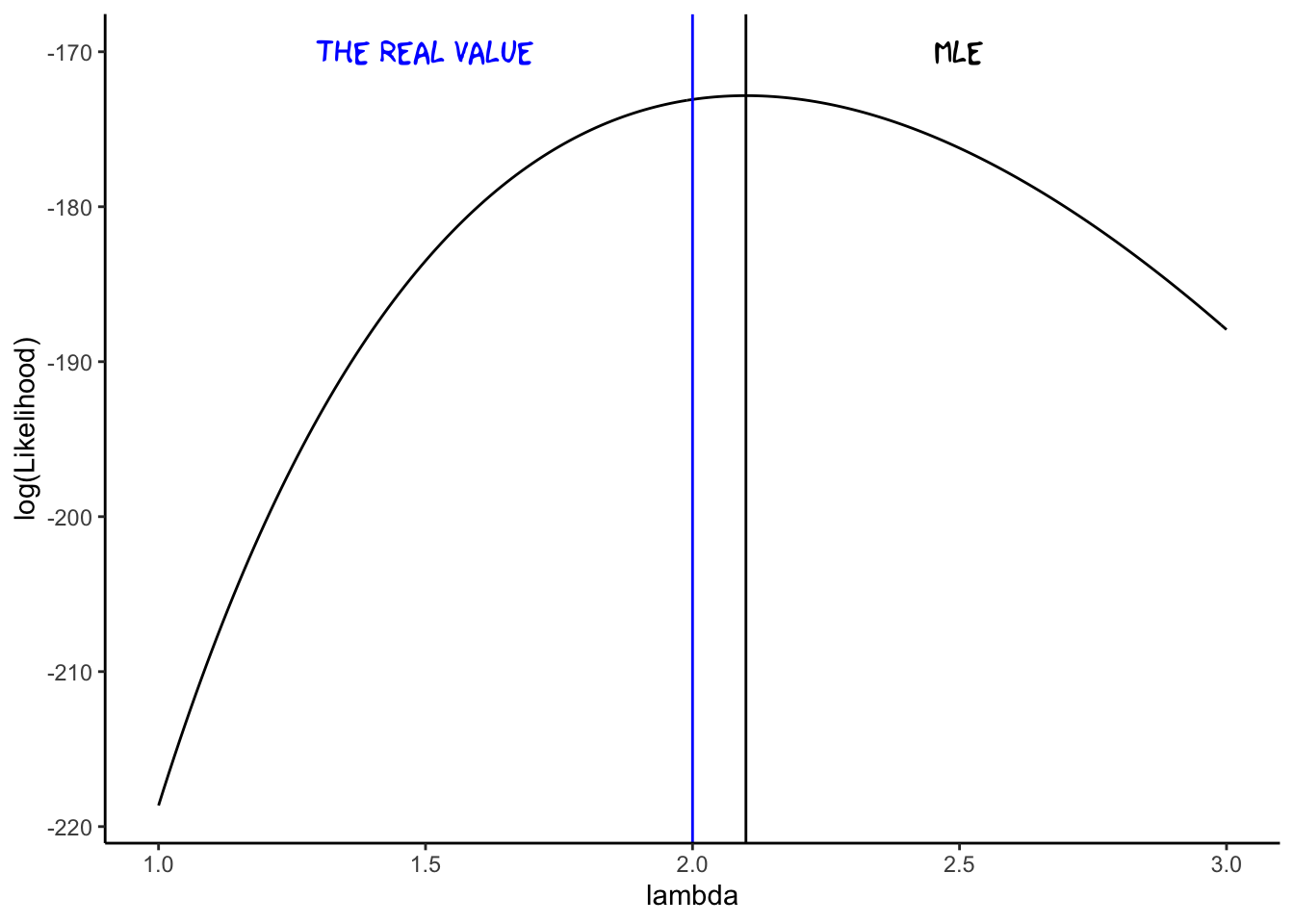
We can also calculate a confidence interval for our estimate. In fact, we should always do this! First we do the approximate one with the 2 SE rule:
sd.data = sd(x)
SE = sd.data/(sqrt(sample.size))
CI.lower = lambda.hat - 2*SE
CI.upper = lambda.hat + 2*SE
print(c(CI.lower,CI.upper))
## [1] 1.815023 2.384977For comparison, we can also use the function t.test (which we will learn more about later):
t.test(x)##
## One Sample t-test
##
## data: x
## t = 14.738, df = 99, p-value < 2.2e-16
## alternative hypothesis: true mean is not equal to 0
## 95 percent confidence interval:
## 1.817272 2.382728
## sample estimates:
## mean of x
## 2.1We find almost the same confidence intervals in both cases. The calculation in the t.test function uses the percentiles of the t-distribution. We can also do this “by hand”:
sd.data = sd(x)
SE = sd.data/(sqrt(sample.size))

alpha = 0.05
CI.lower = lambda.hat + qt(alpha/2,sample.size-1)*SE
CI.upper =  lambda.hat + qt(1-alpha/2,sample.size-1)*SE
print(c(CI.lower,CI.upper))
## [1] 1.817272 2.382728