I discuss a solution to the Monty Hall Problem discussed in the lecture. There are many ways to think of this problem and a thorugh discussion can be found here: https://en.wikipedia.org/wiki/Monty_Hall_problem.
Game Rules:
Pick a door. One door has a prize behind it, say a car, the other two contain just "goats". (Some people might prefer a goat over a car, me included. I just stick with the original formulation here, so let's just say the goat is a symbol for not getting anything and the car a symbol for a prize we actually like to have).
As there are two goats, no matter how you choose, there is at least one goat left among the two remaining doors. The host then reveals a goat behind one of the remaining doors. This means that the opened door is out of the game.
The host offers you to switch doors. You decide whether you want to switch doors or stay with the one you chose. If you switch doors, there is just one door to choose from as one has been removed from the game at step 2.
What should you do?
Let us calculate the chances of winning for the two strategies "switching" and "staying". We use the probabilities in the tree diagrams below. We have one tree diagram to calculate the "switch" strategy's winning chance, and one for the "stay" strategy:
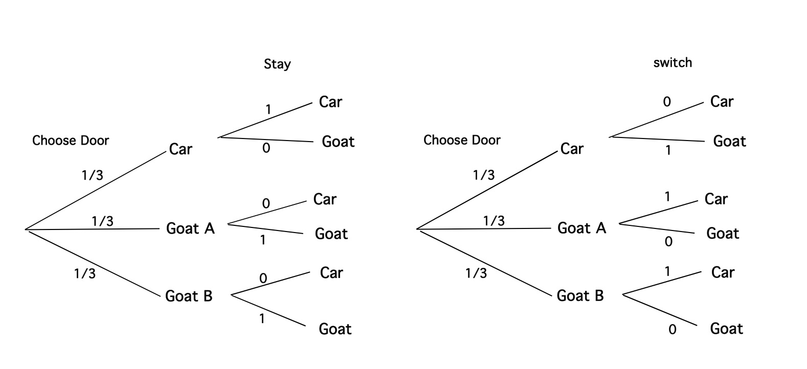
Figure 1: Probability Tree for Monty Hall Problem
The first branches correspond to the "choose initial door" phase. Without any prior information about the doors,the probability that the car is behind the chosen door is 1/3. Now the contestant makes a further choice between switching doors or changing doors.
Let us look at the diagram for staying (left side of Fig. 1). The probability that the car is behind the door unopened by your host depends on which choice you made originally. If the car is behind the door you chose first, the probability that it is behind the other door is 0. If the door you chose first has a goat behind it, then the car is most definitely behind the other door, and the probability that it is behind the door left unopened by your host is 1. We get for the probability to win the car f we stay: \[P(win,stay) = 1/3 \times 1 + 1/3 \times 0 + 1/3 \times 0= 1/3.\] This makes sense, we choose a door randomly and each has the same 1/3 chance of winning. What happens afterwards is not of concern to us as we stick to the originally chosen door. So the only way to win is to chose the right door initially.
Not let us consider what happens if we switch (right side of Fig. 1). The formal calculations now yields: \[P(win,switch) = 1/3 \times 0 + 1/3 \times 1 + 1/3 \times 1 = 2/3.\] This calculation tells us that we would win with a 2/3 probability if we decide to switch. How is that possible? I think it helps to think about this strategy more about a way to force the moderator to give us some crucial information, namely about the location of a bad door. In more technical terms, the sampling space has changed after the opening of the door and it changes differently depending on the first choice of the door. If we choose a goat initially, it is certain that the remaining door is a win, because only one got is left among the two doors. Since it is easier to chose the wrong door initially, we should switch as this would turn a bad - but very likely - initial choice into a good choice.
Here is some R code to illustrate the outcomes of the two strategies (staying and switching) discussed in the lecture. You can copy and paste this code to play around with it.
# number of runs
n = 1000
all.doors = 1:3

# some variables to keep track of waht is going on
win.stay = numeric(n)
win.switch = numeric(n)
chosen = numeric(n)
winning = numeric(n)
openend = numeric(n)

for (i in 1 : n)
{
  # chose a winning door for each time
  winning.door = sample(all.doors,1)

  # contest chooses a door
  chosen.door = sample(all.doors,1)

  # game host opens one door,
  # the remaining door is the one that the contest can switch to
  if(winning.door == chosen.door)
  {
    # we randomly chosen one door that is not the winning door
    # or the chosen door
    # we open the other one
    # the player can switch to the remaining door

    remaining.door = sample(all.doors[-winning.door],1)

  }

  else
  {
    # we select the door that is not the winning door
    # and not the chosen door and open it
    opened.door = all.doors[-c(winning.door,chosen.door)]

    # the remaining door is then the one that is not chosen
    # and not opened
    remaining.door = all.doors[-c(chosen.door,opened.door)]

  }

  win.switch[i] = (remaining.door == winning.door)
  win.stay[i] = (chosen.door == winning.door)

  # record for visualization
  chosen[i] = chosen.door
  winning[i] = winning.door

}
## [1] "The strategy 'switch' yielded 671 wins."## [1] "The strategy 'stay' yielded 329 wins."We can visualize the outcome by plotting when and how often each strategy leads to winning the prize.
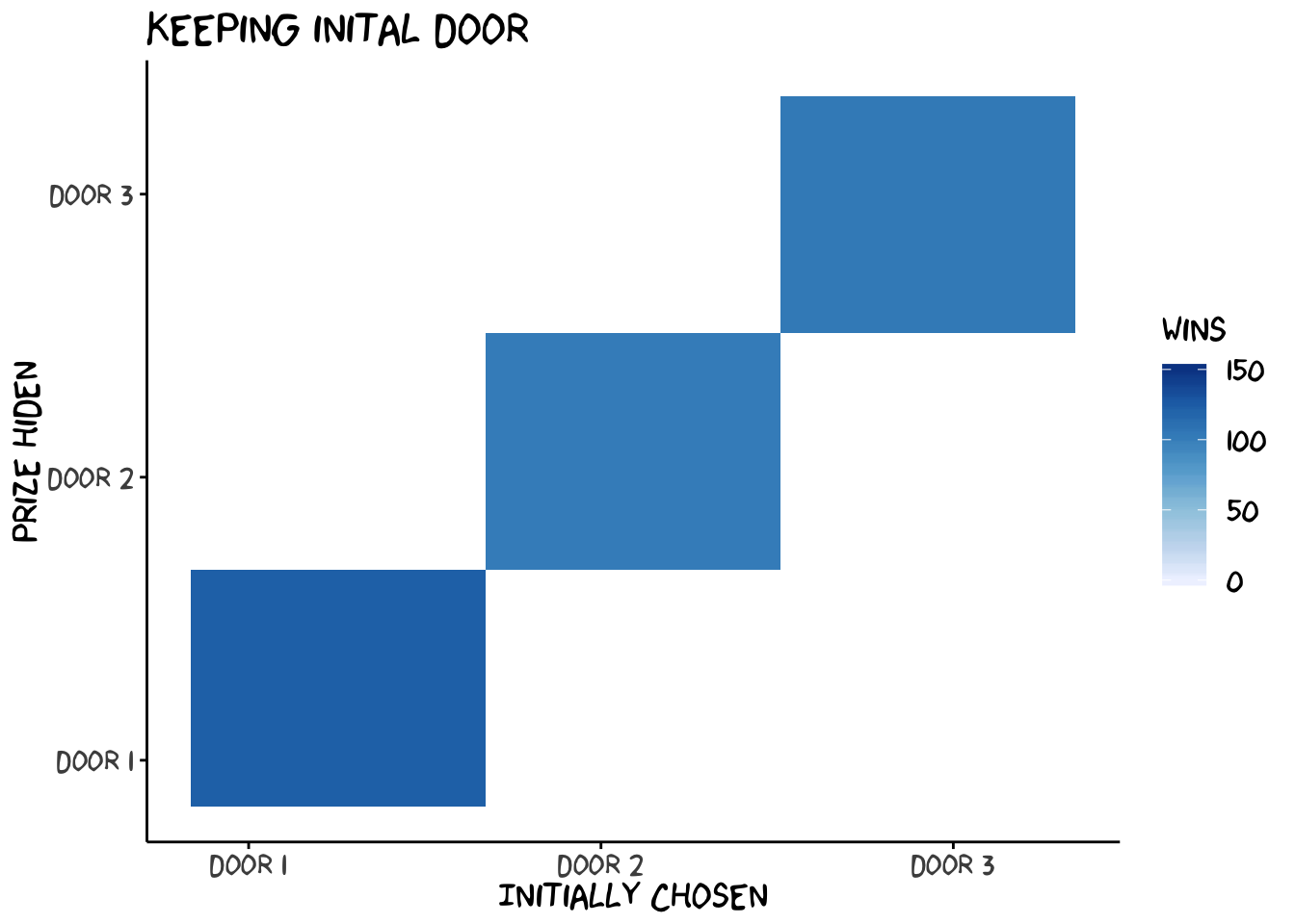
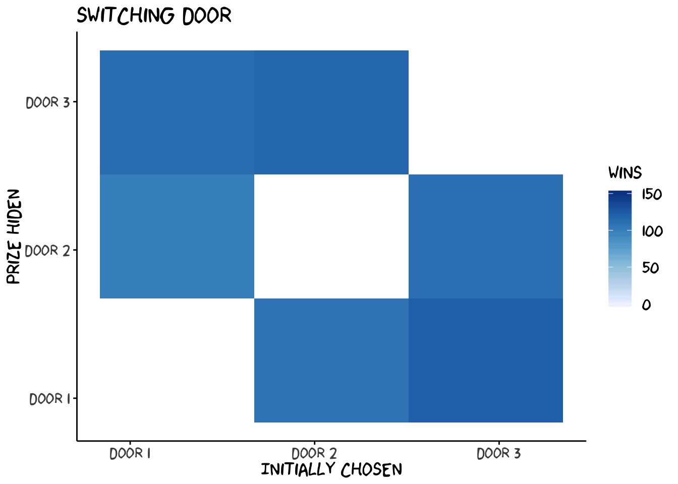
We see two interesting things in this figures: (1) "switch" wins exactly when "stay" doesn't win and (2) switching always wins if you chose the wrong door initially. Thus, staying wins with a probability of 1/3 (choosing the right door out of 3), and switching wins with a probability of 2/3. Exactly as we have calcualted with our decision tree.