We introduce the binomial distribution with a simple example: imagine you have a coin with two sides: Heads and Tails. We don't know if the coin is fair, but we can try to do an experiment to see if it s fair. We flip it many times and if it is a fair coin, we should see the same number of Heads and Tails. Let's say we have flipped it 10 times and got the following sequence: s = {H,T,T,T,H,H,T,H,T,T}. What is the probability for this particular outcome if it is a fair coin? Since all coin tosses are independent, we get:
\[ P(Sequence = s) = (1/2)^{10}. \] W observe that each outcome would be equally likely, because the probability for Heads or Tails are the same: \(1/2\). Clearly this is not very helpful. So let us try something else: we count the number of Heads (calling it a success - the choice that Heads is a success is arbitrary and doesn't matter). In our example the number of heads is
\[H = 4.\]
What is the probability for observing 4 Heads in 10 coin flips? This must be something different than the probability calculated above for one specific sequence, because there are many ways to get 4 Heads. For instance {H,H,H,H,T,T,T,T,T,T} has 4 heads, and so does {H,T,H,T,H,T,H,T,T,T}. Both of these outcomes are equally likely and both of them yield 4 heads.
A next question that naturally arises is whether the probabilities for H = 0, H = 1, etc. are different from each other. Intuitvely one would think so. Let us try to calculate this:
- H = 0
There is only one way to get this outcome, so the probability for this sequence of all Tails is equal to the probability for H = 0:
\[P(H = 0) = (1/2)^{10}.\]
- H = 1
For H = 1, there are 10 possible sequences; the first coin toss is H but all other T, or the second one is H and all other T, or the third one H and all other T, and so on. Thus the probability for H = 1 is \[P(H = 1) = 10*(1/2)^{10},\] because these sequences correspond to disjoint events and we can simply add them up.
- H = k, where k = 0, ..., n
From now on it gets more complex and we do not need to go through all cases separately. Instead we use a result from combinatorics to solve the general case. We need to calculate the number of ways how we can choose k elements out of n, where k is the number of H tosses and n is the total number of tosses. This is given by the so called binomial coefficient:
\[{n\choose k} = \frac{n!}{k!(n-k)!}, \] with \[n! = 1*2*3*...*(n-1)*n.\]
If we now out all this together, we have derived the binomial distribution for the case of \(\pi = 1/2\):
\[ P( H = k) = {n\choose k} (1/2)^n \]
The last step is to consider the general case where \(0 < \pi < 1\), so that the probability for a success is equal to \(\pi\). Then the probability for any sequence with k successes and n-k failures is:
\[\pi^k (1-\pi)^{n-k}\]
and since there are \({n\choose k}\) such sequences the probability for k successes among n trials is: \[P(H = k) = {n\choose k} \pi^k (1-\pi)^{n-k}\]
In R we can get this distribution very easily in the following way (output not shown, copy and paste for trying it).
library(ggplot2)
library(xkcd)
## Loading required package: extrafont## Registering fonts with R# plot the distribution
prob = 0.5
n = 10
k = 0:10
bin.dist = dbinom(k,n,prob)
dat = data.frame(k = k,dist = bin.dist)
ggplot(dat,aes(x = k,y= dist)) +
geom_point(size=5)+
theme_classic() +
theme(text = element_text(size = 30)) And here is a nice version of the plot (all done in R, message me for code): 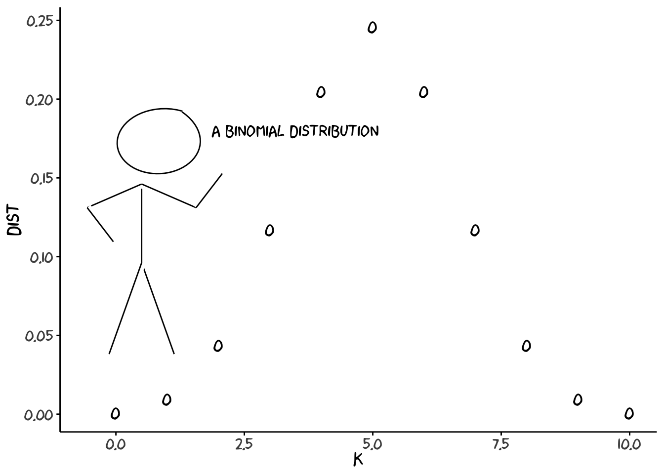 ```
```
If we want to draw a random sample from a distribution, we can also do this in R:
pi = 0.5
n = 10


random.sample = rbinom(1,n,pi)
print(random.sample)
## [1] 4