Consider a medical test for a rare disease. The test is quite accurate: it detects the disease with 95% probability (sensitivity of the test), and indicates the absence of the disease with 90% probability ( specificity of the test).
Notation:
- event D: person has the disease;
- event T: test is positive (i.e., indicates disease)
We assume that the disease has incidence of 1 %: P[D] = 0.01.
You take the test and have a positive result.
What is the probability that you actually have the disease?
We can use Bayes Theorem to calculate this, but how?
We know that the event T (a positive test) has occurred. But what we want to know is the probability for the event D of having the disease. What we are looking for is
P[D|T]
According to Bayes Theorem this can be calculated as
\[ P[D|T] = \frac{P[T|D] P[D]}{P[T]}. \] Let us try to translate this in more common words. The top part is simply the probability of having the disease and a positive test (P[D and T]). The bottom part is the probability to have a positive test. So what we want to calculate is the fraction of positive tests that also have the disease among all positive tests. You can now plug in the numbers using some of the results from the lecture slides and find the answer (see slides pages 35 and 36).
\[ P[T] = 0.1085 \] \[ P[T|D] = 0.95 \] \[ P[D] = 0.01 \]
and finally
\[ P[D|T] = \frac{0.95 * 0.01 }{0.1085} \approx 0.09 \]
So the chance to actually have the disease is pretty low in this case Makes sense, no?
Let us try to put in some numbers to see what is going on here. Assume we test 10 000 people randomly. Of these 10 000 roughly 10 have the disease.
The number of total positive tests will be false positives and true positives. Let us look at the false positives first:
9 990 (the people without the disease) * 0.1 (the probability for a false positive) = 999 false positive results
Now let us look at the true positives:
100 (people with the disease) * 0.95 (sensitivity of the test) = 95 true positives
So we have 95 true positives but 999 false positives and the proportion of true positive results among all positives results is roughly 95/(95+999) \(\approx\) 0.09.
The key point here is that the disease is rare. So even if there is a small chance for a false positive, we expect them to reach large numbers as most tested people do not have the disease. Conversely, the true positive results will be small, because there are only few people with the disease that can yield true positive results. To illustrate this further, let us plot P[D|T] as function of the prevalence P(D):
library(ggplot2)
library(xkcd)
## Loading required package: extrafont## Registering fonts with RpD = seq(0,1,by=0.001)
pTgivenD = 0.95
pTgiven_notD = 0.1
# law of total probability:
pT = pTgivenD * pD + pTgiven_notD*(1-pD)
#Bayes Theorem:
pDgivenT = pTgivenD*pD/pT
dat = data.frame(pT = pD,pDgivenT = pDgivenT)
ggplot(dat,aes(x = pD,y = pDgivenT)) +
geom_line() +
theme_classic() +
xlab("P[D]") +
ylab("P[D|T]") +
theme(text = element_text(size = 25)) 
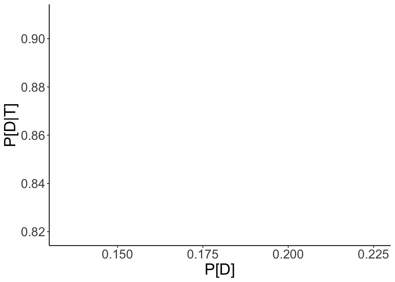
We see that the test’s false positive probability strongly depends on the prevalence. The rarer the disease is, the less reliable the test is in informing you whether you actually have the disease. The specificity also has a strong impact on the interpretation of the test. For instance, for the current Covid-19 PCR tests specificity seems to be closer to 99% than to 90%, then we would get the following:
pD = seq(0,1,by=0.001)
pD =0.18
pTgivenD = 0.87
pTgiven_notD = 1 - 0.97

# law of total probability:
pT =  pTgivenD * pD + pTgiven_notD*(1-pD)

pT
## [1] 0.1812#Bayes Theorem:
pDgivenT = pTgivenD*pD/pT
dat = data.frame(pT = pD,pDgivenT = pDgivenT)
ggplot(dat,aes(x = pD,y = pDgivenT)) +
geom_line() +
theme_classic()+
xlab("P[D]") +
ylab("P[D|T]") +
theme(text = element_text(size = 20)) ## geom_path: Each group consists of only one observation. Do you need to adjust
## the group aesthetic?